
Long-Short Term Memory(LSTM)
LSTM은 RNN의 vanishing, exploding gradient를 완화하기 위해 은닉 상태에 추가로 long term memory를 담당하는 cell state라는 상태를 추가한 모델이다.
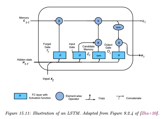
LSTM은 cell state 와 hidden state 를 제어하기 위해 input, output, forgot이라는 3개의 gate를 사용한다. 여기서 input gate 은 입력에서 어떤 정보를 cell state에 추가할지 결정하고, output gate 는 cell state에서 어떤 정보를 다음 hidden state로 보낼지 결정하고, forgot gate 는 cell state에서 어떤 정보를 버릴지를 결정한다.
즉 gating 메커니즘 은 정보의 selection 메커니즘으로 볼 수 있다.
전체 구조는 아래 그림 참조.
LSTM의 다양한 변종이 제안되었는데 10,000개 이상 다른 아키텍쳐에 대한 테스트 결과 일부는 LSTM이나 GRU 보다 더 잘 동작했지만, 일반적으로 LSTM은 대부분의 작업에서 일관되게 잘 작동하는 것으로 나타났다.
Sample Code
아래는 LSTM 모델을 이용해서 분류 문제를 처리하는 간단한 예이다.
만일 분류가 아닌 시퀀스 예측을 수행하려 한다면 아래에서 hidden을 fc에 통과시키는 부분을 시퀀스에 맞게 바꿔서 사용하면 된다.
Model
forget, input, cell, output gate를 갖는 LSTM 모델 코드
class LSTM(nn.Module):
def __init__(self, input_size, hidden_size, num_classes):
super(LSTM, self).__init__()
self.hidden_size = hidden_size
# LSTM 게이트
self.forget_gate = nn.Linear(input_size + hidden_size, hidden_size)
self.input_gate = nn.Linear(input_size + hidden_size, hidden_size)
self.cell_input = nn.Linear(input_size + hidden_size, hidden_size)
self.output_gate = nn.Linear(input_size + hidden_size, hidden_size)
# 활성화 함수
self.sigmoid = nn.Sigmoid()
self.tanh = nn.Tanh()
# 최종 출력을 위한 추가적인 선형 층
self.fc = nn.Linear(hidden_size, num_classes) # 분류 문제를 위한 선형 층
def forward(self, input_seq):
batch_size = input_seq.size(0)
hidden = torch.zeros(batch_size, self.hidden_size)
cell = torch.zeros(batch_size, self.hidden_size)
# sequence 길이만큼 반복
for input_t in input_seq.split(1, dim=1): # sequence 기준으로 split
input_t = input_t.squeeze(1) # 시간 차원을 제거
combined = torch.cat((input_t, hidden), 1) # 배치 차원을 고려하여 결합
# forgot gate, input gate, output gate, cell_input 연산
fg = self.sigmoid(self.forget_gate(combined))
ig = self.sigmoid(self.input_gate(combined))
og = self.sigmoid(self.output_gate(combined))
ci = self.tanh(self.cell_input(combined))
# cell, hidden state 업데이트
cell = fg * cell + ig * ci
hidden = og * self.tanh(cell)
# 마지막 타임스텝의 hidden state를 선형 층에 통과시켜 최종 출력 생성
model_output = self.fc(hidden)
return model_output
Python
복사
Train
다음과 같이 학습할 수 있다. Loss는 모델 출력과 정답 사이의 MSE를 사용한다.
import torch
import torch.nn as nn
import torch.optim as optim
# 하이퍼파라미터 설정
input_size = 5
hidden_size = 10
output_size = 1
num_classes = 5
batch_size = 2
seq_len = 10
# 입력 시퀀스와 대상 시퀀스
input_seq = torch.rand(batch_size, seq_len, input_size)
target_seq = torch.rand(batch_size, output_size)
# 모델 및 하이퍼파라미터 초기화
model = LSTM(input_size, hidden_size, num_classes)
# 손실 함수와 최적화
loss_function = nn.MSELoss()
optimizer = optim.Adam(model.parameters(), lr=0.001)
# 학습 과정
for epoch in range(1000):
optimizer.zero_grad()
model_output = model(input_seq)
loss = loss_function(model_output, target_seq)
loss.backward()
optimizer.step()
if epoch % 100 == 0:
print(f'Epoch: {epoch}, Loss: {loss.item()}')
Python
복사
