AI/ Article/ Annotated Transformer

import os
from os.path import exists
import torch
import torch.nn as nn
from torch.nn.functional import log_softmax, pad
import math
import copy
import time
from torch.optim.lr_scheduler import LambdaLR
import pandas as pd
import altair as alt
from torchtext.data.functional import to_map_style_dataset
from torch.utils.data import DataLoader
from torchtext.vocab import build_vocab_from_iterator
import torchtext.datasets as datasets
import spacy
import GPUtil
import warnings
from torch.utils.data.distributed import DistributedSampler
import torch.distributed as dist
import torch.multiprocessing as mp
from torch.nn.parallel import DistributedDataParallel as DDP


# Set to False to skip notebook execution (e.g. for debugging)
warnings.filterwarnings("ignore")
RUN_EXAMPLES = True
Python
복사

# Some convenience helper functions used throughout the notebook


def is_interactive_notebook():
    return __name__ == "__main__"


def show_example(fn, args=[]):
    if __name__ == "__main__" and RUN_EXAMPLES:
        return fn(*args)


def execute_example(fn, args=[]):
    if __name__ == "__main__" and RUN_EXAMPLES:
        fn(*args)


class DummyOptimizer(torch.optim.Optimizer):
    def __init__(self):
        self.param_groups = [{"lr": 0}]
        None

    def step(self):
        None

    def zero_grad(self, set_to_none=False):
        None


class DummyScheduler:
    def step(self):
        None
Python
복사

Background

순차적 계산을 줄이는 목표는 또한 Extended Neural GPU, ByteNet과 ConvS2S의 기반이 되며, 이들 모두 기본 building block으로 convolutional neural network를 사용하여 모든 입력과 출력 위치에 대해 은닉 표현을 병렬로 계산한다.

이러한 모델들에서 두 임의의 입력 또는 출력 위치 간의 신호를 연호를 연관 시키는데 필요한 연산 수는 ConvS2S의 경우 위치 간 거리에 비례하고, ByteNet의 경우 로그에 비례한다. 이것은 distant(먼) 위치 사이의 의존성을 학습하는데 더 어려움을 만든다. Transformer에서 이것은 상수 연산 수로 줄어들지만 attention 가중치 위치를 평균화 하여 효과적인 해상도가 줄어드는 대신 Multi-Head Attention으로 효과를 상쇄한다.

Self-Attention, 때때로 intra-attention이라 불리는 것은 시퀀스의 표현을 계산하는 측면에서 단일 시퀀스의 다양한 위치를 연관시키는 attention 메커니즘이다. Self-attention은 독해 이해, 요약, 텍스트 추론과 작업-독립적 문장 표현 학습 등을 포함하여 다양한 작업에서 성공적으로 사용되었다. end-to-end 메모리 네트워크는 sequence-aligned recurrence 대신 recurrent attention 메커니즘에 기반하고 단순 언어 질의와 언어 모델링 작업에 대해 잘 수행되었다.

그러나 우리가 아는 한, Transformer는 sequence aligned RNN이나 convolution을 사용하지 않고 self-attention에 전적으로 의존하여 입력과 출력의 표현을 계산하는 첫 번째 transduction 모델이다.

Part 1: Model Architecture

Model Architecture

대부분 경쟁력 있는 neural sequence transduction model은 encoder-decoder 구조를 갖는다. 여기서 인코더는 기호 표현의 입력 시퀀스

(x_1, ..., x_n)

를 연속 표현의 시퀀스

\bold{z} = (z_1, ...,z_n)

로 매핑한다.

\bold{z}

가 주어지면 디코더는 한 번에 하나씩 기호의 출력 시퀀스

(y_1, ...,y_m)

을 생성한다. 각 단계 모델은 auto-regressive이고 다음을 생성할 때 이전에 생성된 기호를 추가 입력으로 흡수한다.

class EncoderDecoder(nn.Module):
    """
    A standard Encoder-Decoder architecture. Base for this and many
    other models.
    """

    def __init__(self, encoder, decoder, src_embed, tgt_embed, generator):
        super(EncoderDecoder, self).__init__()
        self.encoder = encoder
        self.decoder = decoder
        self.src_embed = src_embed
        self.tgt_embed = tgt_embed
        self.generator = generator

    def forward(self, src, tgt, src_mask, tgt_mask):
        "Take in and process masked src and target sequences."
        return self.decode(self.encode(src, src_mask), src_mask, tgt, tgt_mask)

    def encode(self, src, src_mask):
        return self.encoder(self.src_embed(src), src_mask)

    def decode(self, memory, src_mask, tgt, tgt_mask):
        return self.decoder(self.tgt_embed(tgt), memory, src_mask, tgt_mask)
Python
복사

class Generator(nn.Module):
    "Define standard linear + softmax generation step."

    def __init__(self, d_model, vocab):
        super(Generator, self).__init__()
        self.proj = nn.Linear(d_model, vocab)

    def forward(self, x):
        return log_softmax(self.proj(x), dim=-1)
Python
복사

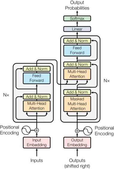
Transformer는 이러한 전반적인 아키텍쳐를 따르며 인코더와 디코더 모두에 대해 self-attention을 쌓고 point-wise 완전 연결된 레이어을 사용한다. 이는 그림 1의 왼쪽과 오른쪽 절반씩 각각 나와 있다.

Encoder and Decoder Stacks

Encoder

이 인코더는

N=6

개의 동일한 레이어의 stack으로 구성된다.

def clones(module, N):
    "Produce N identical layers."
    return nn.ModuleList([copy.deepcopy(module) for _ in range(N)])
Python
복사

class Encoder(nn.Module):
    "Core encoder is a stack of N layers"

    def __init__(self, layer, N):
        super(Encoder, self).__init__()
        self.layers = clones(layer, N)
        self.norm = LayerNorm(layer.size)

    def forward(self, x, mask):
        "Pass the input (and mask) through each layer in turn."
        for layer in self.layers:
            x = layer(x, mask)
        return self.norm(x)
Python
복사

우리는 두 sub-layer의 각각 주위에 residual connection을 사용하고 layer normalization을 수행한다.

class LayerNorm(nn.Module):
    "Construct a layernorm module (See citation for details)."

    def __init__(self, features, eps=1e-6):
        super(LayerNorm, self).__init__()
        self.a_2 = nn.Parameter(torch.ones(features))
        self.b_2 = nn.Parameter(torch.zeros(features))
        self.eps = eps

    def forward(self, x):
        mean = x.mean(-1, keepdim=True)
        std = x.std(-1, keepdim=True)
        return self.a_2 * (x - mean) / (std + self.eps) + self.b_2
Python
복사

즉 각 sub-layer의 출력은

\text{LayerNorm}(x + \text{Sublayer}(x))

이다. 여기서

\text{Sublayer}(x)

는 sub-layer 자체에서 구현되는 함수이다. 우리는 각 sub-layer의 출력에 dropout을 적용한 다음 sub-layer 입력에 더하고 정규화한다.

이 residual connection을 용이하게 하기 위해 모델에서 모든 sub-layer과 embedding layer가

d_\text{model} = 512

차원의 출력을 생성한다.

class SublayerConnection(nn.Module):
    """
    A residual connection followed by a layer norm.
    Note for code simplicity the norm is first as opposed to last.
    """

    def __init__(self, size, dropout):
        super(SublayerConnection, self).__init__()
        self.norm = LayerNorm(size)
        self.dropout = nn.Dropout(dropout)

    def forward(self, x, sublayer):
        "Apply residual connection to any sublayer with the same size."
        return x + self.dropout(sublayer(self.norm(x)))
Python
복사

각 레이어는 두 sub-layer를 갖는다. 첫 번째는 multi-head self-attention 메커니즘이고 두 번째는 단순히 position-wise fully connected feed-forward network이다.

class EncoderLayer(nn.Module):
    "Encoder is made up of self-attn and feed forward (defined below)"

    def __init__(self, size, self_attn, feed_forward, dropout):
        super(EncoderLayer, self).__init__()
        self.self_attn = self_attn
        self.feed_forward = feed_forward
        self.sublayer = clones(SublayerConnection(size, dropout), 2)
        self.size = size

    def forward(self, x, mask):
        "Follow Figure 1 (left) for connections."
        x = self.sublayer[0](x, lambda x: self.self_attn(x, x, x, mask))
        return self.sublayer[1](x, self.feed_forward)
Python
복사

Decoder

디코더 또한

N=6

개의 동일한 레이어의 stack으로 구성된다.

class Decoder(nn.Module):
    "Generic N layer decoder with masking."

    def __init__(self, layer, N):
        super(Decoder, self).__init__()
        self.layers = clones(layer, N)
        self.norm = LayerNorm(layer.size)

    def forward(self, x, memory, src_mask, tgt_mask):
        for layer in self.layers:
            x = layer(x, memory, src_mask, tgt_mask)
        return self.norm(x)
Python
복사

각 인코더 레이어에서 두 sub-layer 외에 디코더는 3번째 sub-layer를 추가한다. 이것은 encoder stack의 출력에 대한 multi-head attention을 수행한다. 인코더와 유사하게 각 sub-layer의 주위에 residual connection을 활용하고 layer normalization을 수행한다.

class DecoderLayer(nn.Module):
    "Decoder is made of self-attn, src-attn, and feed forward (defined below)"

    def __init__(self, size, self_attn, src_attn, feed_forward, dropout):
        super(DecoderLayer, self).__init__()
        self.size = size
        self.self_attn = self_attn
        self.src_attn = src_attn
        self.feed_forward = feed_forward
        self.sublayer = clones(SublayerConnection(size, dropout), 3)

    def forward(self, x, memory, src_mask, tgt_mask):
        "Follow Figure 1 (right) for connections."
        m = memory
        x = self.sublayer[0](x, lambda x: self.self_attn(x, x, x, tgt_mask))
        x = self.sublayer[1](x, lambda x: self.src_attn(x, m, m, src_mask))
        return self.sublayer[2](x, self.feed_forward)
Python
복사

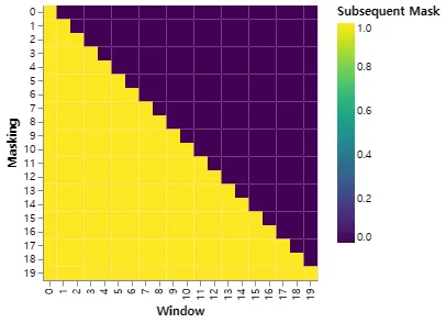
또한 디코더 stack의 self-attention sub-layer를 수정하여 위치가 후속 위치에 attending 하는 것을 방지한다. 이 마스킹은 출력 임베딩이 한 위치로 offset 되어 있다는 사실과 결합되어, 위치

i

에 대한 예측이

i

미만의 위치에서 알려진 출력에만 의존할 수 있도록 한다.

def subsequent_mask(size):
    "Mask out subsequent positions."
    attn_shape = (1, size, size)
    subsequent_mask = torch.triu(torch.ones(attn_shape), diagonal=1).type(
        torch.uint8
    )
    return subsequent_mask == 0
Python
복사

아래 attention mask는 위치 각 tgt 단어 (행)이 참조할 수 있는 위치(column)을 보여준다. 학습하는 동안 단어가 미래 단어에 대해 attending 하는 것을 차단 한다.

def example_mask():
    LS_data = pd.concat(
        [
            pd.DataFrame(
                {
                    "Subsequent Mask": subsequent_mask(20)[0][x, y].flatten(),
                    "Window": y,
                    "Masking": x,
                }
            )
            for y in range(20)
            for x in range(20)
        ]
    )

    return (
        alt.Chart(LS_data)
        .mark_rect()
        .properties(height=250, width=250)
        .encode(
            alt.X("Window:O"),
            alt.Y("Masking:O"),
            alt.Color("Subsequent Mask:Q", scale=alt.Scale(scheme="viridis")),
        )
        .interactive()
    )


show_example(example_mask)
Python
복사

Attention

Attention 함수는 query와 key-value 쌍의 집합을 출력으로 매핑하는 것으로 설명할 수 있다. 여기서 query, keys, values와 출력은 모두 벡터이다. 출력은 values의 weighted sum으로 계산되고 여기서 각 value에 할당되는 weight는 query와 해당하는 key의 compatibility 함수에 의해 계산된다.

우리는 이 특별한 attention을 ‘Scaled Dot-Product Attention’이라 부른다. 입력은

d_k

차원의 queries와 keys와

d_v

차원의 values로 구성된다. 우리는 query를 모든 key와 dot product 하고, 각각을

\sqrt{d_k}

로 나눈 후 softmax 함수를 적용하여 values에 대한 weight를 얻는다.

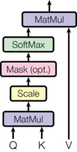
실제로 query의 집합에 대한 attention 함수를 행렬

Q

로 묶어서 동시에 계산한다. keys와 values 또한 행렬

K

와

V

로 묶는다. 출력의 행렬을 다음처럼 계산한다.

\text{Attention}(Q, K,V) = \text{softmax}\left({QK^\top \over \sqrt{d_k}} \right)V

def attention(query, key, value, mask=None, dropout=None):
    "Compute 'Scaled Dot Product Attention'"
    d_k = query.size(-1)
    scores = torch.matmul(query, key.transpose(-2, -1)) / math.sqrt(d_k)
    if mask is not None:
        scores = scores.masked_fill(mask == 0, -1e9)
    p_attn = scores.softmax(dim=-1)
    if dropout is not None:
        p_attn = dropout(p_attn)
    return torch.matmul(p_attn, value), p_attn
Python
복사

두 가지 가장 일반적으로 사용되는 attention 함수는 additive attention과 dot-product(multiplicative) attention이다. dot-product attention은

{1 \over \sqrt{d_k}}

의 스케일링 요소만 제외하면 우리의 알고리즘과 동일하다. additive attention은 단일 hidden layer를 가진 feed-forward network를 사용하여 compatibility 함수를 계산한다. 이론적 복잡성이 유사하지만 dot-product attention이 매우 최적화 되어 있는 행렬 곱 코드를 사용할 수 있기 때문에 실제로 더 빠르고 공간 효율적이다.

d_k

의 값이 작으면 두 가지 메커니즘의 성능이 비슷하지만

d_k

가 클 때는 scaling 없이 dot proudct attention 보다 additive attention은 성능이 더 낫다. 우리는

d_k

의 값이 클 때 dot product의 크기가 커져서 softmax 함수가 극도로 작은 gradient를 갖는 영역으로 밀리는 것으로 추측한다.(dot product가 커지는 이유를 설명하자면,

q

와

k

의 컴포넌트가 평균

0

과 분산

1

인 독립 확률 변수라고 가정하면, 그들의 dot product

q\cdot k = \sum_{i=1}^{d_k} q_ik_i

는 평균

0

, 분산

d_k

를 갖는다) 이 효과를 상쇄하기 위해 우리는 dot product에

{1\over \sqrt{d_k}}

를 곱한다.

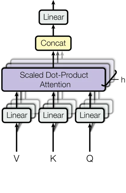
Multi-head attention을 통해 모델은 다양한 위치에서 다양한 표현 부분 공간의 정보에 대해 jointly attend 할 수 있다. 단일 attention head에서는 평균화로 인해 이것이 억제된다.

\text{MultiHead}(Q,K,V) = \text{Concat}(\text{head}_1,...,\text{head}_h)W^O \\ \text{where } \text{head}_i = \text{Attention}(QW_i^Q, KW_i^K, VW_i^V)

여기서 투영은 파라미터 행렬

W_i^Q \in \mathbb{R}^{d_\text{model} \times d_k}, W_i^K \in \mathbb{R}^{d_\text{model} \times d_k}, W_i^V \in \mathbb{R}^{d_\text{model} \times d_v}, W_i^O \in \mathbb{R}^{hd_v \times d_\text{model}}

이다.

이 작업에서 우리는

h=8

개 병렬 attention layer 또는 head를 사용한다. 이들 각각에 대해

d_k = d_v = d_\text{model}/h = 64

를 사용한다. 각 head의 차원이 축소되기 때문에 전체 계산 비용은 전체 차원을 갖춘 single-head attention과 유사하다.

class MultiHeadedAttention(nn.Module):
    def __init__(self, h, d_model, dropout=0.1):
        "Take in model size and number of heads."
        super(MultiHeadedAttention, self).__init__()
        assert d_model % h == 0
        # We assume d_v always equals d_k
        self.d_k = d_model // h
        self.h = h
        self.linears = clones(nn.Linear(d_model, d_model), 4)
        self.attn = None
        self.dropout = nn.Dropout(p=dropout)

    def forward(self, query, key, value, mask=None):
        "Implements Figure 2"
        if mask is not None:
            # Same mask applied to all h heads.
            mask = mask.unsqueeze(1)
        nbatches = query.size(0)

        # 1) Do all the linear projections in batch from d_model => h x d_k
        query, key, value = [
            lin(x).view(nbatches, -1, self.h, self.d_k).transpose(1, 2)
            for lin, x in zip(self.linears, (query, key, value))
        ]

        # 2) Apply attention on all the projected vectors in batch.
        x, self.attn = attention(
            query, key, value, mask=mask, dropout=self.dropout
        )

        # 3) "Concat" using a view and apply a final linear.
        x = (
            x.transpose(1, 2)
            .contiguous()
            .view(nbatches, -1, self.h * self.d_k)
        )
        del query
        del key
        del value
        return self.linears[-1](x)
Python
복사

Applications of Attention in our Model

Transformer는 multi-head attention을 3가지 다른 방식으로 사용한다.

‘encoder-decoder attention’ layer에서 queries는 이전 디코더 레이어에서 오고, memory keys와 values는 인코더의 출력에서 온다. 이를 통해 디코더의 모든 위치가 입력 시퀀스의 모든 위치에 attend 할 수 있다. 이는 sequence-to-sequence 모델에서 일반적인 encoder-decoder attention 메커니즘을 모방한다.

인코더는 self-attention 레이어를 포함한다. self-attention 레이어에서 모든 keys, values와 queries는 동일한 장소, 이 경우에 인코더에서 이전 레이어의 출력에서 온다. 인코더에서 각 위치는 인코더의 이전 레이어에서 모든 위치에 attend 할 수 있다.

유사하게 디코더에서 self-attention 레이어를 통해 디코더에서 각 위치가 해당 위치를 포함하여 디코더의 모든 위치에 attend 할 수 있다. auto-regressive 속성을 보존하기 위해 디코더에서 왼쪽 방향 정보 흐름을 방지해야 한다. 우리는 이를 scaled dot-product attention 내에서 softmax의 입력의 불법적인 연결에 해당하는 모든 값을 masking out(−∞-\infty−∞를 설정하여)하여 구현한다.

Position-wise Feed-Forward Networks

attention sub-layer 외에도 인코더와 디코더의 각 레이어에는 fully connected feed-forward network가 포함된다. 이것은 각 위치에 별도로 동일하게 적용한다. 이것은 중간에 ReLU activation을 갖는 2개 선형 변환으로 구성된다.

\text{FFN}(x) = \max(0, xW_1 + b_1)W_2 + b_2

선형 변환이 다른 위치에서 동일하지만, 레이어마다 다른 파라미터를 사용한다. 이것을 다른 방식으로 설명하면 kernel 크기가

1

인 2개의 convolution이라고 할 수 있다. 입력과 출력의 차원은

d_\text{model} = 512

이고 inner-layer는

d_\text{ff} = 2048

을 갖는다.

class PositionwiseFeedForward(nn.Module):
    "Implements FFN equation."

    def __init__(self, d_model, d_ff, dropout=0.1):
        super(PositionwiseFeedForward, self).__init__()
        self.w_1 = nn.Linear(d_model, d_ff)
        self.w_2 = nn.Linear(d_ff, d_model)
        self.dropout = nn.Dropout(dropout)

    def forward(self, x):
        return self.w_2(self.dropout(self.w_1(x).relu()))
Python
복사

Embeddings and Softmax

다른 시퀀스 transduction 모델과 유사하게, 학습된 임베딩을 사용해서 입력 토큰과 출력 토큰을 차원

d_\text{model}

의 벡터로 변환한다. 또한 일반적인 학습된 선형 변환과 softmax 함수를 사용하여 디코더 출력을 다음 토큰 예측 확률로 변환한다. 우리의 모델에서 두 개의 임베딩 레이어와 pre-softmax 선형 변환 사이에 동일한 가중치 행렬을 공유한다. 임베딩 레이어에서 이러한 가중치에

\sqrt{d_\text{model}}

을 곱한다.

class Embeddings(nn.Module):
    def __init__(self, d_model, vocab):
        super(Embeddings, self).__init__()
        self.lut = nn.Embedding(vocab, d_model)
        self.d_model = d_model

    def forward(self, x):
        return self.lut(x) * math.sqrt(self.d_model)
Python
복사

Positional Encoding

우리의 모델이 recurrence와 convolution을 포함하지 않기 때문에 모델이 시퀀스의 순서를 활용하려면 시퀀스 내 토큰의 상대적 또는 절대적 위치에 관한 정보를 주입해야 한다. 이를 위해 인코더와 디코더 스택의 하단의 입력 임베딩에 ‘positional encoding’을 추가한다. positional encoding의 차원은 임베딩과 동일한

d_\text{model}

이므로 두 값을 더할 수 있다. positional encoding에 대해 학습된 것과 고정된 것 등 많은 선택지가 있다.

이 작업에서 우리는 서로 다른 주파수의 sine, cosine 함수를 사용한다.

\text{PE}_{(\text{pos}, 2i)} = \sin(\text{pos}/10000^{2i/d_\text{model}}) \\\text{PE}_{(\text{pos}, 2i + 1)} = \cos(\text{pos}/10000^{2i/d_\text{model}})

여기서

\text{pos}

는 위치이고

i

는 차원이다. 즉 positional encoding의 각 차원은 sinusoid에 해당한다. 파장은

2\pi

에서

10000 \cdot 2\pi

까지의 등비 수열이다. 우리가 이 함수를 선택한 이유는 임의의 고정된 offset

k

에 대해

PE_{\text{pos+k}}

는

PE_{\text{pos}}

의 선형 함수로써 나타낼 수 있기 때문에, 모델이 상대적 위치에 쉽게 의해 attend 하는 것을 학습할 수 있을 것이라고 가정 했기 때문이다.

또한 인코더와 디코더 stack 모두에서 임베딩과 positional encoding의 합에 dropout을 추가한다. 기본 모델에 대해

P_\text{drop} = 0.1

의 비율을 사용한다.

class PositionalEncoding(nn.Module):
    "Implement the PE function."

    def __init__(self, d_model, dropout, max_len=5000):
        super(PositionalEncoding, self).__init__()
        self.dropout = nn.Dropout(p=dropout)

        # Compute the positional encodings once in log space.
        pe = torch.zeros(max_len, d_model)
        position = torch.arange(0, max_len).unsqueeze(1)
        div_term = torch.exp(
            torch.arange(0, d_model, 2) * -(math.log(10000.0) / d_model)
        )
        pe[:, 0::2] = torch.sin(position * div_term)
        pe[:, 1::2] = torch.cos(position * div_term)
        pe = pe.unsqueeze(0)
        self.register_buffer("pe", pe)

    def forward(self, x):
        x = x + self.pe[:, : x.size(1)].requires_grad_(False)
        return self.dropout(x)
Python
복사

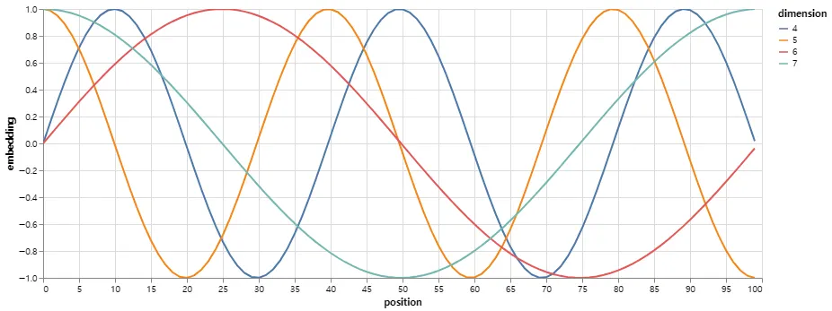
아래 positional encoding은 position에 기반하여 sine 파를 더한다. 파동의 주파수와 offset은 각 차원 마다 다르다.

def example_positional():
    pe = PositionalEncoding(20, 0)
    y = pe.forward(torch.zeros(1, 100, 20))

    data = pd.concat(
        [
            pd.DataFrame(
                {
                    "embedding": y[0, :, dim],
                    "dimension": dim,
                    "position": list(range(100)),
                }
            )
            for dim in [4, 5, 6, 7]
        ]
    )

    return (
        alt.Chart(data)
        .mark_line()
        .properties(width=800)
        .encode(x="position", y="embedding", color="dimension:N")
        .interactive()
    )


show_example(example_positional)
Python
복사

우리는 또한 학습된 positional embedding을 사용하는 것을 실험했고, 두 버전이 거의 동일한 결과를 산출한다는 것을 발견했다. 우리는 sinusoidal 버전을 선택했는데 이는 모델이 학습하는 동안 접한 것보다 더 긴 sequence 길이에 대해 extrapolate 해줄 것이기 때문이다.

Full Model

여기에 전체 모델에 대한 하이퍼파라미터에서 함수를 정의한다.

def make_model(
    src_vocab, tgt_vocab, N=6, d_model=512, d_ff=2048, h=8, dropout=0.1
):
    "Helper: Construct a model from hyperparameters."
    c = copy.deepcopy
    attn = MultiHeadedAttention(h, d_model)
    ff = PositionwiseFeedForward(d_model, d_ff, dropout)
    position = PositionalEncoding(d_model, dropout)
    model = EncoderDecoder(
        Encoder(EncoderLayer(d_model, c(attn), c(ff), dropout), N),
        Decoder(DecoderLayer(d_model, c(attn), c(attn), c(ff), dropout), N),
        nn.Sequential(Embeddings(d_model, src_vocab), c(position)),
        nn.Sequential(Embeddings(d_model, tgt_vocab), c(position)),
        Generator(d_model, tgt_vocab),
    )

    # This was important from their code.
    # Initialize parameters with Glorot / fan_avg.
    for p in model.parameters():
        if p.dim() > 1:
            nn.init.xavier_uniform_(p)
    return model
Python
복사

Inference:

여기서 모델의 예측을 생성하는 forward step을 수행한다. 우리는 transformer를 사용하여 입력을 기억하려고 한다. 보시다시피 모델이 아직 학습되지 않았기 때문에 출력이 무작위로 생성된다. 다음 튜토리얼에서 학습 함수를 만들고 모델이 1에서 10까지의 수를 기억하도록 학습할 것이다.

def inference_test():
    test_model = make_model(11, 11, 2)
    test_model.eval()
    src = torch.LongTensor([[1, 2, 3, 4, 5, 6, 7, 8, 9, 10]])
    src_mask = torch.ones(1, 1, 10)

    memory = test_model.encode(src, src_mask)
    ys = torch.zeros(1, 1).type_as(src)

    for i in range(9):
        out = test_model.decode(
            memory, src_mask, ys, subsequent_mask(ys.size(1)).type_as(src.data)
        )
        prob = test_model.generator(out[:, -1])
        _, next_word = torch.max(prob, dim=1)
        next_word = next_word.data[0]
        ys = torch.cat(
            [ys, torch.empty(1, 1).type_as(src.data).fill_(next_word)], dim=1
        )

    print("Example Untrained Model Prediction:", ys)


def run_tests():
    for _ in range(10):
        inference_test()


show_example(run_tests)

# ---
# Example Untrained Model Prediction: tensor([[0, 0, 0, 0, 0, 0, 0, 0, 0, 0]])
# Example Untrained Model Prediction: tensor([[0, 3, 4, 4, 4, 4, 4, 4, 4, 4]])
# Example Untrained Model Prediction: tensor([[ 0, 10, 10, 10,  3,  2,  5,  7,  9,  6]])
# Example Untrained Model Prediction: tensor([[ 0,  4,  3,  6, 10, 10,  2,  6,  2,  2]])
# Example Untrained Model Prediction: tensor([[ 0,  9,  0,  1,  5, 10,  1,  5, 10,  6]])
# Example Untrained Model Prediction: tensor([[ 0,  1,  5,  1, 10,  1, 10, 10, 10, 10]])
# Example Untrained Model Prediction: tensor([[ 0,  1, 10,  9,  9,  9,  9,  9,  1,  5]])
# Example Untrained Model Prediction: tensor([[ 0,  3,  1,  5, 10, 10, 10, 10, 10, 10]])
# Example Untrained Model Prediction: tensor([[ 0,  3,  5, 10,  5, 10,  4,  2,  4,  2]])
# Example Untrained Model Prediction: tensor([[0, 5, 6, 2, 5, 6, 2, 6, 2, 2]])
Python
복사

Part 2: Model Training

Training

이 섹션은 우리의 모델에 대한 학습 체제를 설명한다.

표준 인코더-디코더 모델을 학습하는데 필요한 몇 가지 도구를 소개하기 위해 잠시 멈춘다. 우선 학습 용 src와 target 문장을 보유하는 batch 객체를 정의하고 mask를 구성한다.

Batches and Masking

class Batch:
    """Object for holding a batch of data with mask during training."""

    def __init__(self, src, tgt=None, pad=2):  # 2 = <blank>
        self.src = src
        self.src_mask = (src != pad).unsqueeze(-2)
        if tgt is not None:
            self.tgt = tgt[:, :-1]
            self.tgt_y = tgt[:, 1:]
            self.tgt_mask = self.make_std_mask(self.tgt, pad)
            self.ntokens = (self.tgt_y != pad).data.sum()

    @staticmethod
    def make_std_mask(tgt, pad):
        "Create a mask to hide padding and future words."
        tgt_mask = (tgt != pad).unsqueeze(-2)
        tgt_mask = tgt_mask & subsequent_mask(tgt.size(-1)).type_as(
            tgt_mask.data
        )
        return tgt_mask
Python
복사

다음으로 loss를 추적하기 위한 일반적인 학습과 scoring 계산 함수를 만든다. 파라미터 업데이트도 처리하는 일반적인 loss 계산 함수를 전달한다.

Training Loop

class TrainState:
    """Track number of steps, examples, and tokens processed"""

    step: int = 0  # Steps in the current epoch
    accum_step: int = 0  # Number of gradient accumulation steps
    samples: int = 0  # total # of examples used
    tokens: int = 0  # total # of tokens processed
Python
복사

def run_epoch(
    data_iter,
    model,
    loss_compute,
    optimizer,
    scheduler,
    mode="train",
    accum_iter=1,
    train_state=TrainState(),
):
    """Train a single epoch"""
    start = time.time()
    total_tokens = 0
    total_loss = 0
    tokens = 0
    n_accum = 0
    for i, batch in enumerate(data_iter):
        out = model.forward(
            batch.src, batch.tgt, batch.src_mask, batch.tgt_mask
        )
        loss, loss_node = loss_compute(out, batch.tgt_y, batch.ntokens)
        # loss_node = loss_node / accum_iter
        if mode == "train" or mode == "train+log":
            loss_node.backward()
            train_state.step += 1
            train_state.samples += batch.src.shape[0]
            train_state.tokens += batch.ntokens
            if i % accum_iter == 0:
                optimizer.step()
                optimizer.zero_grad(set_to_none=True)
                n_accum += 1
                train_state.accum_step += 1
            scheduler.step()

        total_loss += loss
        total_tokens += batch.ntokens
        tokens += batch.ntokens
        if i % 40 == 1 and (mode == "train" or mode == "train+log"):
            lr = optimizer.param_groups[0]["lr"]
            elapsed = time.time() - start
            print(
                (
                    "Epoch Step: %6d | Accumulation Step: %3d | Loss: %6.2f "
                    + "| Tokens / Sec: %7.1f | Learning Rate: %6.1e"
                )
                % (i, n_accum, loss / batch.ntokens, tokens / elapsed, lr)
            )
            start = time.time()
            tokens = 0
        del loss
        del loss_node
    return total_loss / total_tokens, train_state
Python
복사

Training Data and Batching

우리는 약 4.5M 문장 쌍으로 구성된 표준 WMT 2014 English-German 데이터셋으로 학습한다. 문장은 source-target 공유 어휘 크기가 약 37000 토큰인 byte-pair 인코딩을 사용하여 인코딩 되었다. English-French의 경우 36M 문장으로 구성된 훨씬 더 큰 WMT 2014 English-French 데이터셋을 사용했고, 토큰을 32000 단어 조각 어휘 집합으로 분할했다.

문장 쌍은 대략적인 시퀀스 길이에 따라 batch로 묶었다. 각 학습 배치에는 대략 25000개의 source 토큰과 25000개의 target 토큰으로 구성된 문장 쌍의 집합이 포함된다.

Hardware and Schedule

우리는 8개의 NVIDIA P100 GPUs가 장착된 한 대의 머신에서 모델을 학습했다. 그 논문에 내내 설명된 하이퍼파라미터를 사용한 기본 모델의 경우 각 학습 단계는 약 0.4초 걸렸다. 기본 모델은 총 100,000 step(12시간) 동안 학습했다. 대형 모델의 경우 step time은 1.0초가 걸리고 300,000 step(3.5 days) 동안 학습했다.

Optimizer

우리는

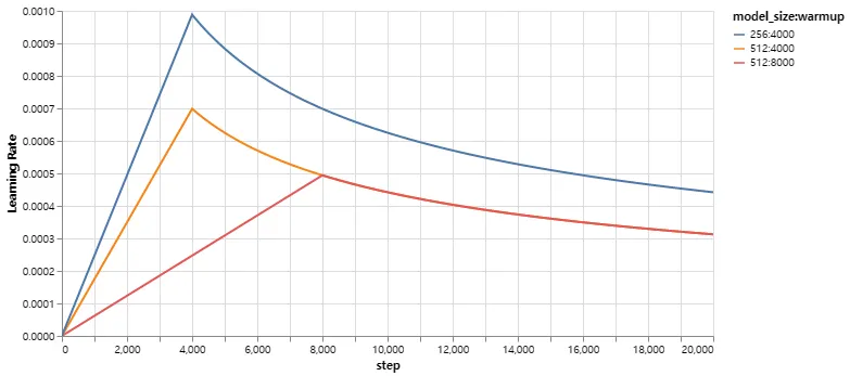
\beta_1 = 0.9, \beta_2 = 0.98, \epsilon = 10^{-9}

의 Adam optimizer를 사용했다. 우리는 학습 과정에서 다음 공식을 따라 학습률을 변화시켰다.

\text{lrate} = d_\text{model}^{-0.5} \cdot \min(\text{step num}^{-0.5},\text{step num} \cdot \text{warmup steps}^{-1.5})

이것은 우선 warmup_steps 학습 단계 동안 학습률을 선형적으로 증가시킨 후, step num의 역 제곱근에 비례하여 감소시키는 것에 해당한다. 우리는

\text{warmup steps} = 4000

을 사용했다.

이 부분은 매우 중요하다. 이 모델 설정으로 학습해야 한다.

다양한 모델 크기와 최적화 하이퍼파라미터에 대한 이 모델 커브의 예이다.

def rate(step, model_size, factor, warmup):
    """
    we have to default the step to 1 for LambdaLR function
    to avoid zero raising to negative power.
    """
    if step == 0:
        step = 1
    return factor * (
        model_size ** (-0.5) * min(step ** (-0.5), step * warmup ** (-1.5))
    )
Python
복사

def example_learning_schedule():
    opts = [
        [512, 1, 4000],  # example 1
        [512, 1, 8000],  # example 2
        [256, 1, 4000],  # example 3
    ]

    dummy_model = torch.nn.Linear(1, 1)
    learning_rates = []

    # we have 3 examples in opts list.
    for idx, example in enumerate(opts):
        # run 20000 epoch for each example
        optimizer = torch.optim.Adam(
            dummy_model.parameters(), lr=1, betas=(0.9, 0.98), eps=1e-9
        )
        lr_scheduler = LambdaLR(
            optimizer=optimizer, lr_lambda=lambda step: rate(step, *example)
        )
        tmp = []
        # take 20K dummy training steps, save the learning rate at each step
        for step in range(20000):
            tmp.append(optimizer.param_groups[0]["lr"])
            optimizer.step()
            lr_scheduler.step()
        learning_rates.append(tmp)

    learning_rates = torch.tensor(learning_rates)

    # Enable altair to handle more than 5000 rows
    alt.data_transformers.disable_max_rows()

    opts_data = pd.concat(
        [
            pd.DataFrame(
                {
                    "Learning Rate": learning_rates[warmup_idx, :],
                    "model_size:warmup": ["512:4000", "512:8000", "256:4000"][
                        warmup_idx
                    ],
                    "step": range(20000),
                }
            )
            for warmup_idx in [0, 1, 2]
        ]
    )

    return (
        alt.Chart(opts_data)
        .mark_line()
        .properties(width=600)
        .encode(x="step", y="Learning Rate", color="model_size:warmup:N")
        .interactive()
    )


example_learning_schedule()
Python
복사

Regularization

Label Smoothing

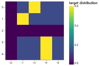
학습하는 동안 우리는

\epsilon_\text{ls} = 0.1

값의 label smoothing을 이용했다. 이것은 모델이 더 불확실해지도록 학습하기 떄문에 perplexity에는 해가 되지만 정확도와 BLEU score를 개선한다.

우리는 KL div loss를 사용하여 label smoothing을 구현한다. one-hot target 분포를 사용하는 대신, 정답 단어에 대한 confidence(신뢰도)와 어휘 집합 도처에 분포된 나머지 smoothing 질량을 생성한다.

class LabelSmoothing(nn.Module):
    "Implement label smoothing."

    def __init__(self, size, padding_idx, smoothing=0.0):
        super(LabelSmoothing, self).__init__()
        self.criterion = nn.KLDivLoss(reduction="sum")
        self.padding_idx = padding_idx
        self.confidence = 1.0 - smoothing
        self.smoothing = smoothing
        self.size = size
        self.true_dist = None

    def forward(self, x, target):
        assert x.size(1) == self.size
        true_dist = x.data.clone()
        true_dist.fill_(self.smoothing / (self.size - 2))
        true_dist.scatter_(1, target.data.unsqueeze(1), self.confidence)
        true_dist[:, self.padding_idx] = 0
        mask = torch.nonzero(target.data == self.padding_idx)
        if mask.dim() > 0:
            true_dist.index_fill_(0, mask.squeeze(), 0.0)
        self.true_dist = true_dist
        return self.criterion(x, true_dist.clone().detach())
Python
복사

여기서 신뢰도에 따라 질량이 단어에 어떻게 분포되는지에 대한 예를 볼 수 있다.

# Example of label smoothing.
def example_label_smoothing():
    crit = LabelSmoothing(5, 0, 0.4)
    predict = torch.FloatTensor(
        [
            [0, 0.2, 0.7, 0.1, 0],
            [0, 0.2, 0.7, 0.1, 0],
            [0, 0.2, 0.7, 0.1, 0],
            [0, 0.2, 0.7, 0.1, 0],
            [0, 0.2, 0.7, 0.1, 0],
        ]
    )
    crit(x=predict.log(), target=torch.LongTensor([2, 1, 0, 3, 3]))
    LS_data = pd.concat(
        [
            pd.DataFrame(
                {
                    "target distribution": crit.true_dist[x, y].flatten(),
                    "columns": y,
                    "rows": x,
                }
            )
            for y in range(5)
            for x in range(5)
        ]
    )

    return (
        alt.Chart(LS_data)
        .mark_rect(color="Blue", opacity=1)
        .properties(height=200, width=200)
        .encode(
            alt.X("columns:O", title=None),
            alt.Y("rows:O", title=None),
            alt.Color(
                "target distribution:Q", scale=alt.Scale(scheme="viridis")
            ),
        )
        .interactive()
    )


show_example(example_label_smoothing)
Python
복사

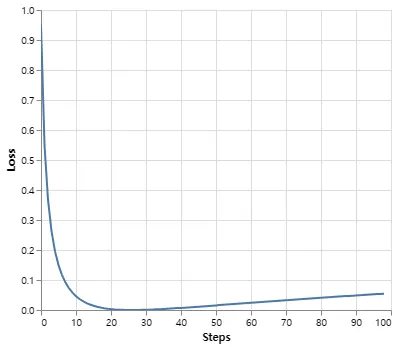
Label smoothing은 실제로 주어진 선택에 매우 확신을 가지면 모델에 페널티를 부여한다.

def loss(x, crit):
    d = x + 3 * 1
    predict = torch.FloatTensor([[0, x / d, 1 / d, 1 / d, 1 / d]])
    return crit(predict.log(), torch.LongTensor([1])).data


def penalization_visualization():
    crit = LabelSmoothing(5, 0, 0.1)
    loss_data = pd.DataFrame(
        {
            "Loss": [loss(x, crit) for x in range(1, 100)],
            "Steps": list(range(99)),
        }
    ).astype("float")

    return (
        alt.Chart(loss_data)
        .mark_line()
        .properties(width=350)
        .encode(
            x="Steps",
            y="Loss",
        )
        .interactive()
    )


show_example(penalization_visualization)
Python
복사

A First Example

단순 복사 작업을 시도하는 것에서 시작한다. 작은 어휘에서 무작위 입력 기호 집합이 주어지면, 목표는 동일한 기호를 생성하는 것이다.

Synthetic Data

def data_gen(V, batch_size, nbatches):
    "Generate random data for a src-tgt copy task."
    for i in range(nbatches):
        data = torch.randint(1, V, size=(batch_size, 10))
        data[:, 0] = 1
        src = data.requires_grad_(False).clone().detach()
        tgt = data.requires_grad_(False).clone().detach()
        yield Batch(src, tgt, 0)
Python
복사

Loss Computation

class SimpleLossCompute:
    "A simple loss compute and train function."

    def __init__(self, generator, criterion):
        self.generator = generator
        self.criterion = criterion

    def __call__(self, x, y, norm):
        x = self.generator(x)
        sloss = (
            self.criterion(
                x.contiguous().view(-1, x.size(-1)), y.contiguous().view(-1)
            )
            / norm
        )
        return sloss.data * norm, sloss
Python
복사

Greedy Decoding

이 코드는 단순성을 위해 greedy 디코딩을 사용하여 변형을 예측한다.

def greedy_decode(model, src, src_mask, max_len, start_symbol):
    memory = model.encode(src, src_mask)
    ys = torch.zeros(1, 1).fill_(start_symbol).type_as(src.data)
    for i in range(max_len - 1):
        out = model.decode(
            memory, src_mask, ys, subsequent_mask(ys.size(1)).type_as(src.data)
        )
        prob = model.generator(out[:, -1])
        _, next_word = torch.max(prob, dim=1)
        next_word = next_word.data[0]
        ys = torch.cat(
            [ys, torch.zeros(1, 1).type_as(src.data).fill_(next_word)], dim=1
        )
    return ys
Python
복사

# Train the simple copy task.
def example_simple_model():
    V = 11
    criterion = LabelSmoothing(size=V, padding_idx=0, smoothing=0.0)
    model = make_model(V, V, N=2)

    optimizer = torch.optim.Adam(
        model.parameters(), lr=0.5, betas=(0.9, 0.98), eps=1e-9
    )
    lr_scheduler = LambdaLR(
        optimizer=optimizer,
        lr_lambda=lambda step: rate(
            step, model_size=model.src_embed[0].d_model, factor=1.0, warmup=400
        ),
    )

    batch_size = 80
    for epoch in range(20):
        model.train()
        run_epoch(
            data_gen(V, batch_size, 20),
            model,
            SimpleLossCompute(model.generator, criterion),
            optimizer,
            lr_scheduler,
            mode="train",
        )
        model.eval()
        run_epoch(
            data_gen(V, batch_size, 5),
            model,
            SimpleLossCompute(model.generator, criterion),
            DummyOptimizer(),
            DummyScheduler(),
            mode="eval",
        )[0]

    model.eval()
    src = torch.LongTensor([[0, 1, 2, 3, 4, 5, 6, 7, 8, 9]])
    max_len = src.shape[1]
    src_mask = torch.ones(1, 1, max_len)
    print(greedy_decode(model, src, src_mask, max_len=max_len, start_symbol=0))


# execute_example(example_simple_model)
Python
복사

Part 3: A Real World Example

이제 Multi30k German-English 번역 작업을 사용하여 실제 예제를 고려하자. 이 작업은 논문에서 고려한 WMT 작업에 비해 훨씬 작은 작업지만 전체 시스템을 설명한다. 또한 multi-gpu 프로세싱을 사용하여 속도를 높이는 방법을 보인다.

Data Loading

토큰화를 위해 torchtext와 spacy를 사용하여 dataset을 로드한다.

# Load spacy tokenizer models, download them if they haven't been
# downloaded already
def load_tokenizers():

    try:
        spacy_de = spacy.load("de_core_news_sm")
    except IOError:
        os.system("python -m spacy download de_core_news_sm")
        spacy_de = spacy.load("de_core_news_sm")

    try:
        spacy_en = spacy.load("en_core_web_sm")
    except IOError:
        os.system("python -m spacy download en_core_web_sm")
        spacy_en = spacy.load("en_core_web_sm")

    return spacy_de, spacy_en
Python
복사

def tokenize(text, tokenizer):
    return [tok.text for tok in tokenizer.tokenizer(text)]


def yield_tokens(data_iter, tokenizer, index):
    for from_to_tuple in data_iter:
        yield tokenizer(from_to_tuple[index])
Python
복사

def build_vocabulary(spacy_de, spacy_en):
    def tokenize_de(text):
        return tokenize(text, spacy_de)

    def tokenize_en(text):
        return tokenize(text, spacy_en)

    print("Building German Vocabulary ...")
    train, val, test = datasets.Multi30k(language_pair=("de", "en"))
    vocab_src = build_vocab_from_iterator(
        yield_tokens(train + val + test, tokenize_de, index=0),
        min_freq=2,
        specials=["<s>", "</s>", "<blank>", "<unk>"],
    )

    print("Building English Vocabulary ...")
    train, val, test = datasets.Multi30k(language_pair=("de", "en"))
    vocab_tgt = build_vocab_from_iterator(
        yield_tokens(train + val + test, tokenize_en, index=1),
        min_freq=2,
        specials=["<s>", "</s>", "<blank>", "<unk>"],
    )

    vocab_src.set_default_index(vocab_src["<unk>"])
    vocab_tgt.set_default_index(vocab_tgt["<unk>"])

    return vocab_src, vocab_tgt


def load_vocab(spacy_de, spacy_en):
    if not exists("vocab.pt"):
        vocab_src, vocab_tgt = build_vocabulary(spacy_de, spacy_en)
        torch.save((vocab_src, vocab_tgt), "vocab.pt")
    else:
        vocab_src, vocab_tgt = torch.load("vocab.pt")
    print("Finished.\nVocabulary sizes:")
    print(len(vocab_src))
    print(len(vocab_tgt))
    return vocab_src, vocab_tgt


if is_interactive_notebook():
    # global variables used later in the script
    spacy_de, spacy_en = show_example(load_tokenizers)
    vocab_src, vocab_tgt = show_example(load_vocab, args=[spacy_de, spacy_en])
Python
복사

배치 크기는 속도에 큰 영향을 미친다. 우리는 최소한의 패딩으로 매우 균일하게 분할된 배치를 갖기를 원한다. 이를 위해 default torchtext 배치 방식을 약간 해킹해야 한다. 이 코드는 default batching을 패치하여 tight한 배치를 찾기에 충분한 문장을 search하도록 한다.

Iterators

def collate_batch(
    batch,
    src_pipeline,
    tgt_pipeline,
    src_vocab,
    tgt_vocab,
    device,
    max_padding=128,
    pad_id=2,
):
    bs_id = torch.tensor([0], device=device)  # <s> token id
    eos_id = torch.tensor([1], device=device)  # </s> token id
    src_list, tgt_list = [], []
    for (_src, _tgt) in batch:
        processed_src = torch.cat(
            [
                bs_id,
                torch.tensor(
                    src_vocab(src_pipeline(_src)),
                    dtype=torch.int64,
                    device=device,
                ),
                eos_id,
            ],
            0,
        )
        processed_tgt = torch.cat(
            [
                bs_id,
                torch.tensor(
                    tgt_vocab(tgt_pipeline(_tgt)),
                    dtype=torch.int64,
                    device=device,
                ),
                eos_id,
            ],
            0,
        )
        src_list.append(
            # warning - overwrites values for negative values of padding - len
            pad(
                processed_src,
                (
                    0,
                    max_padding - len(processed_src),
                ),
                value=pad_id,
            )
        )
        tgt_list.append(
            pad(
                processed_tgt,
                (0, max_padding - len(processed_tgt)),
                value=pad_id,
            )
        )

    src = torch.stack(src_list)
    tgt = torch.stack(tgt_list)
    return (src, tgt)
Python
복사

def create_dataloaders(
    device,
    vocab_src,
    vocab_tgt,
    spacy_de,
    spacy_en,
    batch_size=12000,
    max_padding=128,
    is_distributed=True,
):
    # def create_dataloaders(batch_size=12000):
    def tokenize_de(text):
        return tokenize(text, spacy_de)

    def tokenize_en(text):
        return tokenize(text, spacy_en)

    def collate_fn(batch):
        return collate_batch(
            batch,
            tokenize_de,
            tokenize_en,
            vocab_src,
            vocab_tgt,
            device,
            max_padding=max_padding,
            pad_id=vocab_src.get_stoi()["<blank>"],
        )

    train_iter, valid_iter, test_iter = datasets.Multi30k(
        language_pair=("de", "en")
    )

    train_iter_map = to_map_style_dataset(
        train_iter
    )  # DistributedSampler needs a dataset len()
    train_sampler = (
        DistributedSampler(train_iter_map) if is_distributed else None
    )
    valid_iter_map = to_map_style_dataset(valid_iter)
    valid_sampler = (
        DistributedSampler(valid_iter_map) if is_distributed else None
    )

    train_dataloader = DataLoader(
        train_iter_map,
        batch_size=batch_size,
        shuffle=(train_sampler is None),
        sampler=train_sampler,
        collate_fn=collate_fn,
    )
    valid_dataloader = DataLoader(
        valid_iter_map,
        batch_size=batch_size,
        shuffle=(valid_sampler is None),
        sampler=valid_sampler,
        collate_fn=collate_fn,
    )
    return train_dataloader, valid_dataloader
Python
복사

Training the System

def train_worker(
    gpu,
    ngpus_per_node,
    vocab_src,
    vocab_tgt,
    spacy_de,
    spacy_en,
    config,
    is_distributed=False,
):
    print(f"Train worker process using GPU: {gpu} for training", flush=True)
    torch.cuda.set_device(gpu)

    pad_idx = vocab_tgt["<blank>"]
    d_model = 512
    model = make_model(len(vocab_src), len(vocab_tgt), N=6)
    model.cuda(gpu)
    module = model
    is_main_process = True
    if is_distributed:
        dist.init_process_group(
            "nccl", init_method="env://", rank=gpu, world_size=ngpus_per_node
        )
        model = DDP(model, device_ids=[gpu])
        module = model.module
        is_main_process = gpu == 0

    criterion = LabelSmoothing(
        size=len(vocab_tgt), padding_idx=pad_idx, smoothing=0.1
    )
    criterion.cuda(gpu)

    train_dataloader, valid_dataloader = create_dataloaders(
        gpu,
        vocab_src,
        vocab_tgt,
        spacy_de,
        spacy_en,
        batch_size=config["batch_size"] // ngpus_per_node,
        max_padding=config["max_padding"],
        is_distributed=is_distributed,
    )

    optimizer = torch.optim.Adam(
        model.parameters(), lr=config["base_lr"], betas=(0.9, 0.98), eps=1e-9
    )
    lr_scheduler = LambdaLR(
        optimizer=optimizer,
        lr_lambda=lambda step: rate(
            step, d_model, factor=1, warmup=config["warmup"]
        ),
    )
    train_state = TrainState()

    for epoch in range(config["num_epochs"]):
        if is_distributed:
            train_dataloader.sampler.set_epoch(epoch)
            valid_dataloader.sampler.set_epoch(epoch)

        model.train()
        print(f"[GPU{gpu}] Epoch {epoch} Training ====", flush=True)
        _, train_state = run_epoch(
            (Batch(b[0], b[1], pad_idx) for b in train_dataloader),
            model,
            SimpleLossCompute(module.generator, criterion),
            optimizer,
            lr_scheduler,
            mode="train+log",
            accum_iter=config["accum_iter"],
            train_state=train_state,
        )

        GPUtil.showUtilization()
        if is_main_process:
            file_path = "%s%.2d.pt" % (config["file_prefix"], epoch)
            torch.save(module.state_dict(), file_path)
        torch.cuda.empty_cache()

        print(f"[GPU{gpu}] Epoch {epoch} Validation ====", flush=True)
        model.eval()
        sloss = run_epoch(
            (Batch(b[0], b[1], pad_idx) for b in valid_dataloader),
            model,
            SimpleLossCompute(module.generator, criterion),
            DummyOptimizer(),
            DummyScheduler(),
            mode="eval",
        )
        print(sloss)
        torch.cuda.empty_cache()

    if is_main_process:
        file_path = "%sfinal.pt" % config["file_prefix"]
        torch.save(module.state_dict(), file_path)
Python
복사

def train_distributed_model(vocab_src, vocab_tgt, spacy_de, spacy_en, config):
    from the_annotated_transformer import train_worker

    ngpus = torch.cuda.device_count()
    os.environ["MASTER_ADDR"] = "localhost"
    os.environ["MASTER_PORT"] = "12356"
    print(f"Number of GPUs detected: {ngpus}")
    print("Spawning training processes ...")
    mp.spawn(
        train_worker,
        nprocs=ngpus,
        args=(ngpus, vocab_src, vocab_tgt, spacy_de, spacy_en, config, True),
    )


def train_model(vocab_src, vocab_tgt, spacy_de, spacy_en, config):
    if config["distributed"]:
        train_distributed_model(
            vocab_src, vocab_tgt, spacy_de, spacy_en, config
        )
    else:
        train_worker(
            0, 1, vocab_src, vocab_tgt, spacy_de, spacy_en, config, False
        )


def load_trained_model():
    config = {
        "batch_size": 32,
        "distributed": False,
        "num_epochs": 8,
        "accum_iter": 10,
        "base_lr": 1.0,
        "max_padding": 72,
        "warmup": 3000,
        "file_prefix": "multi30k_model_",
    }
    model_path = "multi30k_model_final.pt"
    if not exists(model_path):
        train_model(vocab_src, vocab_tgt, spacy_de, spacy_en, config)

    model = make_model(len(vocab_src), len(vocab_tgt), N=6)
    model.load_state_dict(torch.load("multi30k_model_final.pt"))
    return model


if is_interactive_notebook():
    model = load_trained_model()
Python
복사

모델이 학습되면 디코드하여 일련의 번역의 생성할 수 있다. 여기서는 간단히 validation set에서 첫 문장을 번역한다. 이 데이터셋은 꽤 작고 따라서 greedy search를 사용하는 번역은 꽤 정확하다.

Additional Components: BPE, Search, Averaging

따라서 이것은 대부분 transformer 모델 그 자체를 다룬다. 우리가 명시적으로 다루지 않은 4가지 측면이 존재한다. OpenNMT-py에 이 추가적인 기능들이 모두 포함되어 있다.

BPE/Word-piece: 우리는 라이브러리를 사용하여 우선 데이터를 subword 단위로 전처리 할 수 있다. Rico Sennrich의 subword-nmt 구현 참조. 이런 모델은 학습 데이터를 다음과 같이 변환한다.

▁Die ▁Protokoll datei ▁kann ▁ heimlich ▁per ▁E - Mail ▁oder ▁FTP ▁an ▁einen ▁bestimmte n ▁Empfänger ▁gesendet ▁werden .
Python
복사

Shared Embeddings: 공유된 어휘를 갖는 BPE를 사용할 때 source, target, generator 사이에 동일한 가중치 벡터를 공유할 수 있다. 이것을 모델에 추가하기 위해 간단히 다음과 같이 수행할 수 있다.

if False:
    model.src_embed[0].lut.weight = model.tgt_embeddings[0].lut.weight
    model.generator.lut.weight = model.tgt_embed[0].lut.weight
Python
복사

Beam Search: 이것은 여기서 다루기엔 너무 복잡하다. pytorch 구현에 대해 OpenNMT-py 참조

Model Averaging: 논문은 앙상블 효과를 생성하기 위해 마지막 k개 체크포인트를 평균화했다. 모델이 여러 개인 경우 사후에 이 작업을 수행 할 수 있다.

def average(model, models):
    "Average models into model"
    for ps in zip(*[m.params() for m in [model] + models]):
        ps[0].copy_(torch.sum(*ps[1:]) / len(ps[1:]))
Python
복사

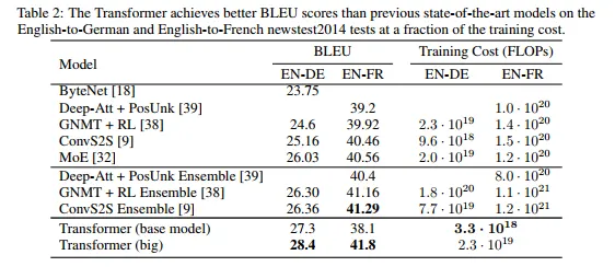
Results

WMT 2014 English-to-German 번역 작업에서 big transformer 모델(표 2의 Transformer (big))은 이전에 보고된 최고의 모델(앙상블 포함)보다 2.0 BLEU 이상 높은 28.4라는 최신 성능을 달성했다. 이 모델의 구성은 표 3의 마지막에 나열되어 있다. 학습에는 8개의 P100 GPU에서 3.5일이 걸렸다. 우리의 기본 모델 조차 경쟁 모델 중 어떤 것보다 훈련 비용이 적음에도 이전에 발표된 모든 모델과 앙상블을 surpasses(능가했다)

WMT 2014 English-to-French 번역 작업에서 우리의 big 모델은 41.0의 BLEU 점수를 달성했고 이전에 발표된 모든 단일 모델을 능가했으면서도 학습 비용은 1/4 미만이었다. English-to-French에 대해 학습된 Tranformer (big) 모델에서는 dropout 비율을

0.3

대신

P_\text{drop} = 0.1

을 사용했다.

마지막 섹션의 추가 확장을 사용하여 OpenNMT-py 복제가 EN-DE WMT에서 26.9에 도달했다. 여기서는 재구현을 위해 파라미터를 로드했다.

# Load data and model for output checks
def check_outputs(
    valid_dataloader,
    model,
    vocab_src,
    vocab_tgt,
    n_examples=15,
    pad_idx=2,
    eos_string="</s>",
):
    results = [()] * n_examples
    for idx in range(n_examples):
        print("\nExample %d ========\n" % idx)
        b = next(iter(valid_dataloader))
        rb = Batch(b[0], b[1], pad_idx)
        greedy_decode(model, rb.src, rb.src_mask, 64, 0)[0]

        src_tokens = [
            vocab_src.get_itos()[x] for x in rb.src[0] if x != pad_idx
        ]
        tgt_tokens = [
            vocab_tgt.get_itos()[x] for x in rb.tgt[0] if x != pad_idx
        ]

        print(
            "Source Text (Input)        : "
            + " ".join(src_tokens).replace("\n", "")
        )
        print(
            "Target Text (Ground Truth) : "
            + " ".join(tgt_tokens).replace("\n", "")
        )
        model_out = greedy_decode(model, rb.src, rb.src_mask, 72, 0)[0]
        model_txt = (
            " ".join(
                [vocab_tgt.get_itos()[x] for x in model_out if x != pad_idx]
            ).split(eos_string, 1)[0]
            + eos_string
        )
        print("Model Output               : " + model_txt.replace("\n", ""))
        results[idx] = (rb, src_tokens, tgt_tokens, model_out, model_txt)
    return results


def run_model_example(n_examples=5):
    global vocab_src, vocab_tgt, spacy_de, spacy_en

    print("Preparing Data ...")
    _, valid_dataloader = create_dataloaders(
        torch.device("cpu"),
        vocab_src,
        vocab_tgt,
        spacy_de,
        spacy_en,
        batch_size=1,
        is_distributed=False,
    )

    print("Loading Trained Model ...")

    model = make_model(len(vocab_src), len(vocab_tgt), N=6)
    model.load_state_dict(
        torch.load("multi30k_model_final.pt", map_location=torch.device("cpu"))
    )

    print("Checking Model Outputs:")
    example_data = check_outputs(
        valid_dataloader, model, vocab_src, vocab_tgt, n_examples=n_examples
    )
    return model, example_data


# execute_example(run_model_example)
Python
복사

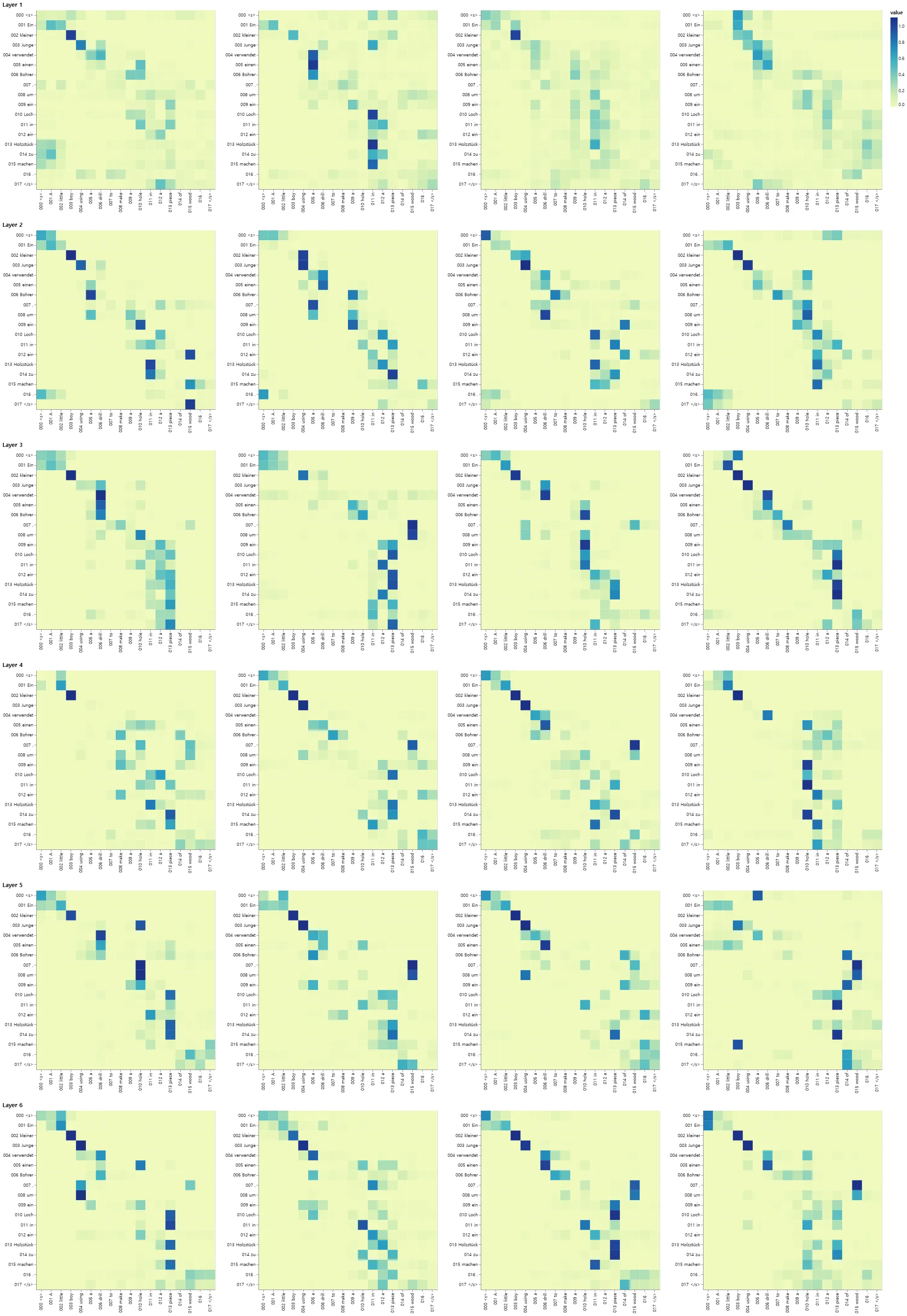
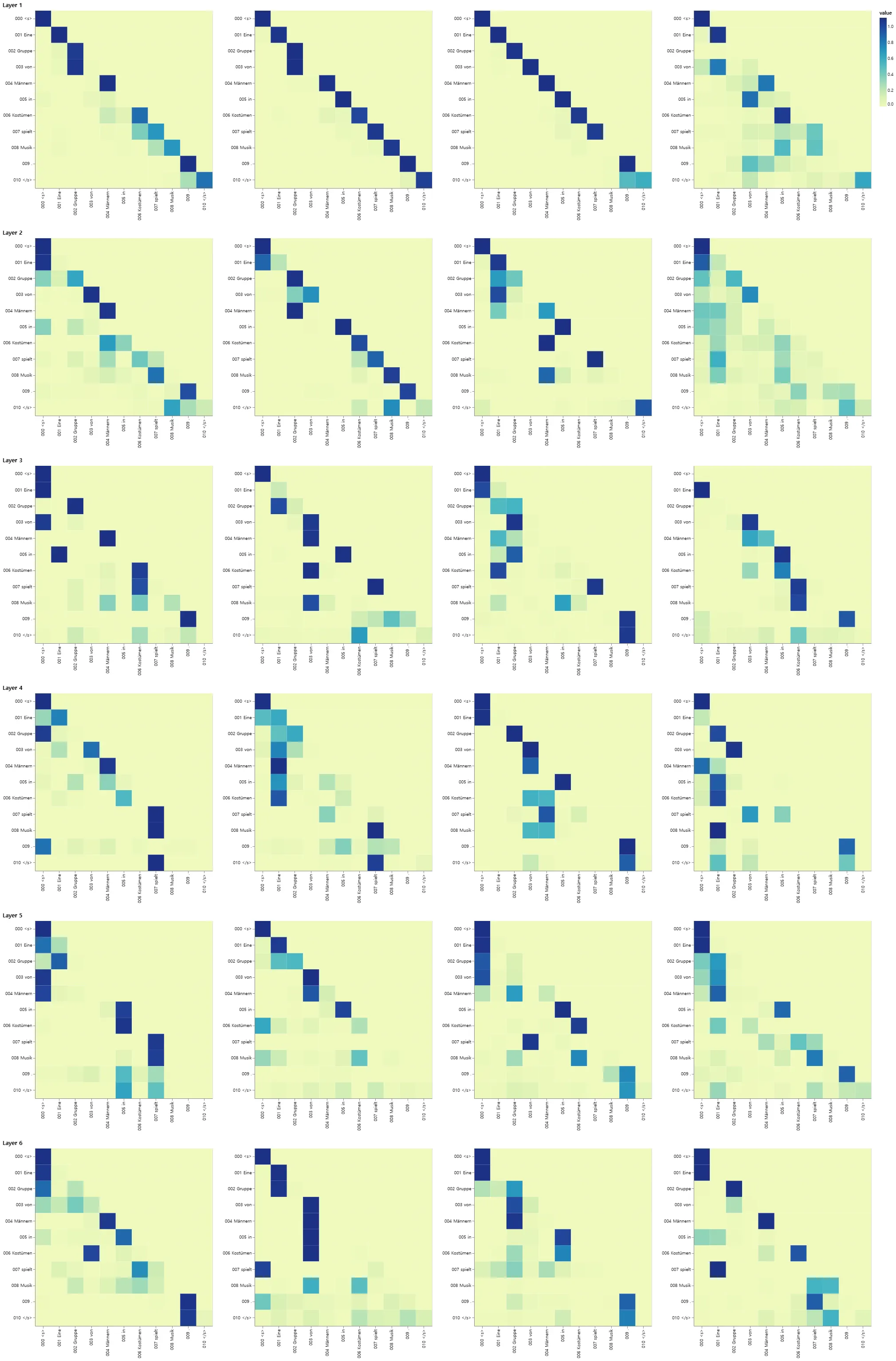
Attention Visualization

greedy 디코더를 사용하더라도 번역도 꽤 좋아 보인다. attention의 각 레이어에서 무슨 일이 벌어지고 있는지를 확인하기 위해 시각화할 수 있다.

def mtx2df(m, max_row, max_col, row_tokens, col_tokens):
    "convert a dense matrix to a data frame with row and column indices"
    return pd.DataFrame(
        [
            (
                r,
                c,
                float(m[r, c]),
                "%.3d %s"
                % (r, row_tokens[r] if len(row_tokens) > r else "<blank>"),
                "%.3d %s"
                % (c, col_tokens[c] if len(col_tokens) > c else "<blank>"),
            )
            for r in range(m.shape[0])
            for c in range(m.shape[1])
            if r < max_row and c < max_col
        ],
        # if float(m[r,c]) != 0 and r < max_row and c < max_col],
        columns=["row", "column", "value", "row_token", "col_token"],
    )


def attn_map(attn, layer, head, row_tokens, col_tokens, max_dim=30):
    df = mtx2df(
        attn[0, head].data,
        max_dim,
        max_dim,
        row_tokens,
        col_tokens,
    )
    return (
        alt.Chart(data=df)
        .mark_rect()
        .encode(
            x=alt.X("col_token", axis=alt.Axis(title="")),
            y=alt.Y("row_token", axis=alt.Axis(title="")),
            color="value",
            tooltip=["row", "column", "value", "row_token", "col_token"],
        )
        .properties(height=400, width=400)
        .interactive()
    )
Python
복사

def get_encoder(model, layer):
    return model.encoder.layers[layer].self_attn.attn


def get_decoder_self(model, layer):
    return model.decoder.layers[layer].self_attn.attn


def get_decoder_src(model, layer):
    return model.decoder.layers[layer].src_attn.attn


def visualize_layer(model, layer, getter_fn, ntokens, row_tokens, col_tokens):
    # ntokens = last_example[0].ntokens
    attn = getter_fn(model, layer)
    n_heads = attn.shape[1]
    charts = [
        attn_map(
            attn,
            0,
            h,
            row_tokens=row_tokens,
            col_tokens=col_tokens,
            max_dim=ntokens,
        )
        for h in range(n_heads)
    ]
    assert n_heads == 8
    return alt.vconcat(
        charts[0]
        # | charts[1]
        | charts[2]
        # | charts[3]
        | charts[4]
        # | charts[5]
        | charts[6]
        # | charts[7]
        # layer + 1 due to 0-indexing
    ).properties(title="Layer %d" % (layer + 1))
Python
복사

Encoder Self Attention

def viz_encoder_self():
    model, example_data = run_model_example(n_examples=1)
    example = example_data[
        len(example_data) - 1
    ]  # batch object for the final example

    layer_viz = [
        visualize_layer(
            model, layer, get_encoder, len(example[1]), example[1], example[1]
        )
        for layer in range(6)
    ]
    return alt.hconcat(
        layer_viz[0]
        # & layer_viz[1]
        & layer_viz[2]
        # & layer_viz[3]
        & layer_viz[4]
        # & layer_viz[5]
    )


show_example(viz_encoder_self)
Python
복사

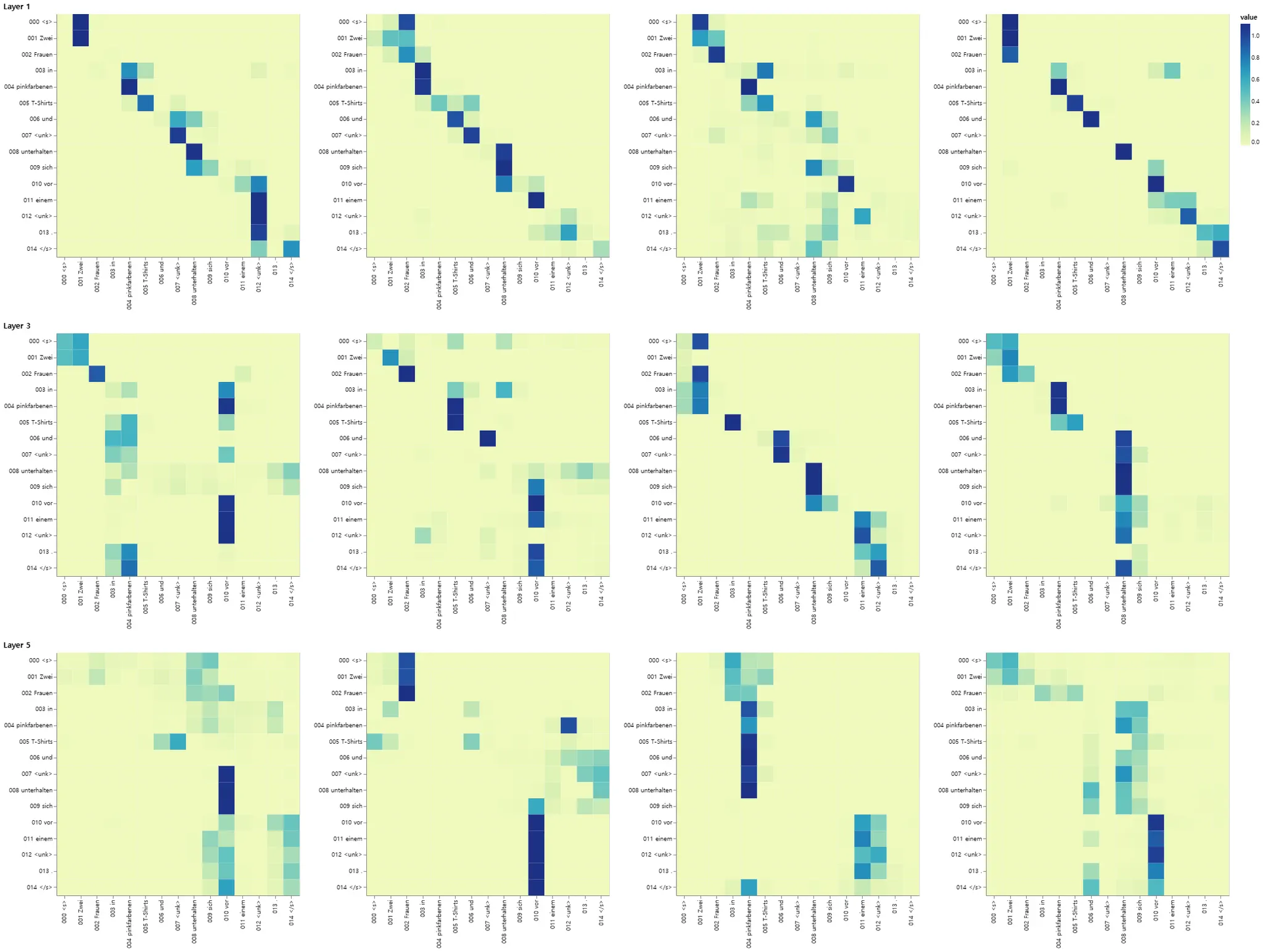
Decoder Self Attention

def viz_decoder_self():
    model, example_data = run_model_example(n_examples=1)
    example = example_data[len(example_data) - 1]

    layer_viz = [
        visualize_layer(
            model,
            layer,
            get_decoder_self,
            len(example[1]),
            example[1],
            example[1],
        )
        for layer in range(6)
    ]
    return alt.hconcat(
        layer_viz[0]
        & layer_viz[1]
        & layer_viz[2]
        & layer_viz[3]
        & layer_viz[4]
        & layer_viz[5]
    )


show_example(viz_decoder_self)
Python
복사

Decoder Src Attention

def viz_decoder_src():
    model, example_data = run_model_example(n_examples=1)
    example = example_data[len(example_data) - 1]

    layer_viz = [
        visualize_layer(
            model,
            layer,
            get_decoder_src,
            max(len(example[1]), len(example[2])),
            example[1],
            example[2],
        )
        for layer in range(6)
    ]
    return alt.hconcat(
        layer_viz[0]
        & layer_viz[1]
        & layer_viz[2]
        & layer_viz[3]
        & layer_viz[4]
        & layer_viz[5]
    )


show_example(viz_decoder_src)
Python
복사