AI/ Consistency Model

Consistency Model

Consistency Model은 Diffusion 모델의 수십-수천 단계가 필요한 느린 샘플링 속도를 개선하는 모델로 one-step 만으로 샘플링을 생성 할 수 있게 한다. 물론 샘플 품질을 높이기 위해 더 많은 단계를 사용하는 것도 가능하다. 여러 면에서 Consistency Model을 Pre-trained Diffusion 모델로 Distilling을 이용하여 학습하게 되면 Diffusion 모델의 확장이라고 할 수 있지만, 만일 Consistency Model을 Standalone으로 학습하면 독립적인 생성 모델이라 할 수 있다.

Consistency Model은 diffusion 샘플링 궤적에서 임의의 중간 noisy 데이터 포인트

\bold{x}_t, t> 0

을 원본

\bold{x}_0

에 직접 매핑하는 방법을 학습한다. 동일한 궤적에 있는 데이터 포인트가 모두 동일한 원점에 매핑되는 self-consistency라는 속성 때문에 consistency model이라 불린다.

중간 noisy 데이터 포인트에서 원본을 직접 매핑하기 때문에 1 step만으로 샘플을 생성할 수 있고 따라서 기존 DDPM이나 DDIM에 비해 매우 빠른 샘플링이 가능하면서도 높은 품질을 유지할 수 있다.

궤적

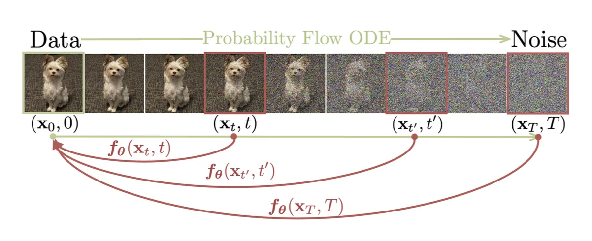
\{\mathbf{x}_t \vert t \in [\epsilon, T]\}

이 주어지면 consistency 함수

f

는

f: (\mathbf{x}_t, t) \mapsto \mathbf{x}_\epsilon

로 정의되고 등식

f(\mathbf{x}_t, t) = f(\mathbf{x}_{t’}, t’) = \mathbf{x}_\epsilon

는 모든

t, t’ \in [\epsilon, T]

에 대해 참이다.

t=\epsilon

이면

f

는 항등 함수이다. 모델은 다음과 같이 파라미터화 될 수 있다. 여기서

c_\text{skip}(t)

와

c_\text{out}(t)

함수는

c_\text{skip}(\epsilon) = 1, c_\text{out}(\epsilon) = 0

인 방법으로 설계된다.

f_\theta(\mathbf{x}, t) = c_\text{skip}(t)\mathbf{x} + c_\text{out}(t) F_\theta(\mathbf{x}, t)

consistency 모델은 multi-step 샘플링 프로세스를 따라 더 나은 품질을 위해 trading computation의 유연성을 유지하면서 단일 step으로 샘플을 생성할 수 있다.

consistency 모델을 학습하는 방법은 2가지가 존재한다. consistency distillation(CD)라 부르는 방법은 pre-trained diffusion 모델을 이용해서 distillation 하는 방법이고, consistency training(CT)라 부르는 방법은 consistency model 단독으로 학습하는 방법이다. 이 방법의 경우 consistency model은 diffusion 모델과는 다른 새로운 형태의 생성 모델이 된다.

Consistency Distillation (CD)

consistency distillation(CD) 방법은 pre-trained diffusion 모델을 이용하여 distillation 하는 학습 방법으로, 동일한 궤적에서 생성된 쌍에 대한 모델 출력 사이의 차이를 최소화하여 diffusion 모델을 consistency 모델로 distill 한다. 이를 통해 훨씬 더 저렴한 샘플링 평가가 가능하다. consistency distillation loss는 다음과 같다.

\begin{aligned} \mathcal{L}^N_\text{CD} (\theta, \theta^-; \phi) &= \mathbb{E} [\lambda(t_n)d(f_\theta(\mathbf{x}_{t_{n+1}}, t_{n+1}), f_{\theta^-}(\hat{\mathbf{x}}^\phi_{t_n}, t_n)] \\ \hat{\mathbf{x}}^\phi_{t_n} &= \mathbf{x}_{t_{n+1}} - (t_n - t_{n+1}) \Phi(\mathbf{x}_{t_{n+1}}, t_{n+1}; \phi) \end{aligned}

여기서

•

Φ(.;ϕ)\Phi(.;\phi)Φ(.;ϕ)는 one-step ODE solver의 업데이트 함수이다.

•

n∼U[1,N−1]n \sim \mathcal{U}[1, N-1]n∼U[1,N−1]는 1,…,N−11, \dots, N-11,…,N−1에 대한 균등 분포를 갖는다.

•

네트워크 파라미터 θ−\theta^-θ−는 학습을 매우 안정 시키는 θ\thetaθ의 EMA 버전이다.(DQN 또는 momentum contrastive learning 같은)

•

d(.,.)d(.,.)d(.,.)는 ℓ2\ell_2ℓ2​, ℓ1\ell_1ℓ1​ 또는 LPIPS(learned perceptual image patch similarity) 거리 같이 ∀x,y:d(x,y)≤0\forall \mathbf{x}, \mathbf{y}: d(\mathbf{x}, \mathbf{y}) \leq 0∀x,y:d(x,y)≤0이고 d(x,y)=0d(\mathbf{x}, \mathbf{y}) = 0d(x,y)=0이면 x=y\mathbf{x} = \mathbf{y}x=y이고 iff를 만족하는 positive distance metric 함수이다. 

•

λ(.)∈R+\lambda(.) \in \mathbb{R}^+λ(.)∈R+는 positive weighting 함수이고 논문에서는 λ(tn)=1\lambda(t_n)=1λ(tn​)=1을 설정했다.

Consistency Training (CT)

다른 옵션은 pre-trained diffusion 모델 없이 consistency 모델을 독립적으로 훈련하는 것이다. CD에서는 pre-trained score model

s_\phi(\mathbf{x}, t)

이 ground truth score

\nabla\log p_t(\mathbf{x})

를 근사하기 위해 사용되지만 CT에서는 이 score 함수를 추정하는 방법이 필요하고

\nabla\log p_t(\mathbf{x})

의 비편향 추정기가

-\frac{\mathbf{x}_t - \mathbf{x}}{t^2}

로 존재한다는 것이 밝혀졌다. CT loss는 다음처럼 정의된다.

\mathcal{L}^N_\text{CT} (\theta, \theta^-; \phi) = \mathbb{E}[\lambda(t_n)d(f_\theta(\mathbf{x} + t_{n+1} \mathbf{z},\;t_{n+1}), f_{\theta^-}(\mathbf{x} + t_n \mathbf{z},\;t_n)]\\\text{ where }\mathbf{z} \in \mathcal{N}(\mathbf{0}, \mathbf{I})

실험에 따라 다음이 발견됐다.

•

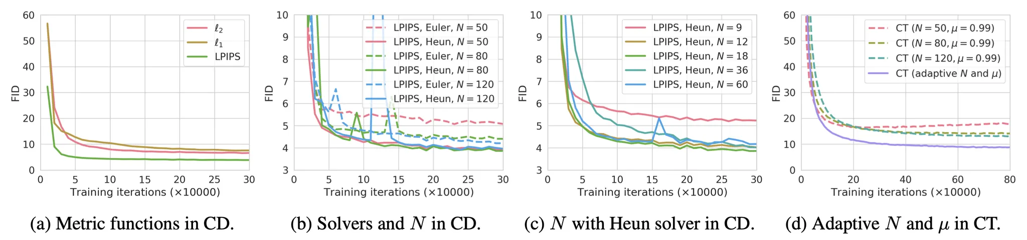
고차 ODE solver가 동일한 NNN에서 더 작은 추정 에러를 갖기 때문에 Heun ODE solver가 Euler’s first-order solver 보다 잘 작동한다. 

•

거리 메트릭 함수 d(.)d(.)d(.)의 다양한 옵션 사이에서 LPIPS 메트릭은 ℓ1\ell_1ℓ1​과 ℓ2\ell_2ℓ2​ 거리보다 더 잘 작동했다.

•

NNN이 작을수록 수렴이 빨라지지만 샘플은 나쁘고, NNN이 클수록 수렴은 느려지지만 수렴시 샘플은 더 좋아진다.

Sample Code

이하 코드는 Consistency Model 논문에 구현된 코드를 참조한다. Diffusion 모델 동일하기 때문에 Model과 학습 코드는 생략.

Sampling

모델의 예측과 입력 사이의 scale을 조정하여 최종 denoise 결과를 생성하는

f_\theta(\mathbf{x}, t) = c_\text{skip}(t)\mathbf{x} + c_\text{out}(t) F_\theta(\mathbf{x}, t)

에 해당하는 코드는 아래처럼 구성된다. 이것은 기존의 progressive distillation에서 입력과 노이즈의 scale을 조정하는

\bold{z}_t = \alpha_t\bold{x} + \sigma_t \boldsymbol{\epsilon}

를 개선한 것이다.

def denoise(self, model, x_t, sigmas, **model_kwargs):
    import torch.distributed as dist

    if not self.distillation:
        c_skip, c_out, c_in = [
            append_dims(x, x_t.ndim) for x in self.get_scalings(sigmas)
        ]
    else:
        c_skip, c_out, c_in = [
            append_dims(x, x_t.ndim)
            for x in self.get_scalings_for_boundary_condition(sigmas)
        ]
    rescaled_t = 1000 * 0.25 * th.log(sigmas + 1e-44)
    # x_t는 batch에서 가져온 여러 장의 이미지이고 각각의 time schedule에 맞게 noisy 된 상태
    model_output = model(c_in * x_t, rescaled_t, **model_kwargs)
    denoised = c_out * model_output + c_skip * x_t
    return model_output, denoised
Python
복사

Objective

Consistency Distillation, Consistency Training Loss

Consistency Distillation(CD)은 pre-trained diffusion 모델을 이용해서 consistency 모델을 distilling으로 학습하는 방법이고 Consistency Training(CT)은 pre-trained diffusion 모델 없이 consistency model을 단독으로 학습하는 방법이다.

Consistency Distillation(CD)에서는 teacher 모델을 이용해서 학습이 수행되고, Consistency Training(CT)에서는 target 모델을 이용해서 학습이 수행된다. CD에서는 teacher 모델을 이용하여 heun_solver()을 사용해서 denoise를 예측하고, CT에서는 euler_solver() —teacher model 없는—을 수행한 후에 target 모델을 이용하여 denoise를 수행한다.

time schedule 별로 noise가 적용된 이미지에 대해 denoise를 예측하고 그 loss에 대해 time schedule 별 weight를 적용하여 최종 loss를 계산 하므로, 모델은 주어진 noisy 이미지와 time step 정보를 이용하여 이미지를 어떻게 원본으로 한 번에 복구할 지를 학습하게 된다.

def consistency_losses(
    self,
    model,
    x_start,
    num_scales,
    model_kwargs=None,
    target_model=None,
    teacher_model=None,
    teacher_diffusion=None,
    noise=None,
):
    if model_kwargs is None:
        model_kwargs = {}
    if noise is None:
        noise = th.randn_like(x_start)

    dims = x_start.ndim

    def denoise_fn(x, t):
        return self.denoise(model, x, t, **model_kwargs)[1]

    if target_model:

        @th.no_grad()
        def target_denoise_fn(x, t):
            return self.denoise(target_model, x, t, **model_kwargs)[1]

    else:
        raise NotImplementedError("Must have a target model")

    if teacher_model:

        @th.no_grad()
        def teacher_denoise_fn(x, t):
            return teacher_diffusion.denoise(teacher_model, x, t, **model_kwargs)[1]

    @th.no_grad()
    # heun solver는 예측과 수정 2번 수행한다.
    def heun_solver(samples, t, next_t, x0):
        x = samples
        if teacher_model is None:
            denoiser = x0
        else:
            denoiser = teacher_denoise_fn(x, t)

        d = (x - denoiser) / append_dims(t, dims)
        samples = x + d * append_dims(next_t - t, dims)
        
        if teacher_model is None:
            denoiser = x0
        else:
            denoiser = teacher_denoise_fn(samples, next_t)

        next_d = (samples - denoiser) / append_dims(next_t, dims)
        samples = x + (d + next_d) * append_dims((next_t - t) / 2, dims)

        return samples

    @th.no_grad()
    def euler_solver(samples, t, next_t, x0):
        x = samples
        if teacher_model is None:
            denoiser = x0
        else:
            denoiser = teacher_denoise_fn(x, t)
        d = (x - denoiser) / append_dims(t, dims)
        samples = x + d * append_dims(next_t - t, dims)

        return samples

		# 무작위 index 벡터 생성
    indices = th.randint(
        0, num_scales - 1, (x_start.shape[0],), device=x_start.device
    )

		# 무작위 index를 바탕으로 time schedule 벡터 계산
    t = self.sigma_max ** (1 / self.rho) + indices / (num_scales - 1) * (
        self.sigma_min ** (1 / self.rho) - self.sigma_max ** (1 / self.rho)
    )
    t = t**self.rho

		# index에 1을 더해서 t 다음의 time schedule 값을 생성
    t2 = self.sigma_max ** (1 / self.rho) + (indices + 1) / (num_scales - 1) * (
        self.sigma_min ** (1 / self.rho) - self.sigma_max ** (1 / self.rho)
    )
    t2 = t2**self.rho

		# batch에서 뽑은 여러 이미지(x_start)에 대해 time schedule 별로 노이즈를 적용하여 noisy 입력(x_t)를 생성
    x_t = x_start + noise * append_dims(t, dims)

		# get_rng_state()/set_rng_state()은 확률적 요소의 일관성을 유지하기 위해 사용한다.
    dropout_state = th.get_rng_state()  # 현재 랜덤 넘버 생성기의 상태를 가져온다.
    
		# 학습 중인 모델로 denoise 예측
    distiller = denoise_fn(x_t, t)

    if teacher_model is None:
		    # Consistency Training
        x_t2 = euler_solver(x_t, t, t2, x_start).detach()
    else:
		    # Consistency Distillation으로 denoise 예측
        x_t2 = heun_solver(x_t, t, t2, x_start).detach()

    th.set_rng_state(dropout_state)  # 저장된 랜덤 넘버 생성기의 상태를 다시 설정한다.
    
		# Consistency Distillation. target 모델을 이용해서 denoise 예측
    distiller_target = target_denoise_fn(x_t2, t2)
    distiller_target = distiller_target.detach()

		# 각 시간 단계에 대한 신호대 잡음비(snr) 계산
    snrs = self.get_snr(t)
    
    # snr을 이용하여 time schedule 별로 가중치 계산
    weights = get_weightings(self.weight_schedule, snrs, self.sigma_data)
    
    # 현재 모델의 예측과 target 사이의 loss 계산
    # time schedule 별로 loss가 계산 되도록 loss에 가중치를 곱한다.
    if self.loss_norm == "l1":
        diffs = th.abs(distiller - distiller_target)
        loss = mean_flat(diffs) * weights
    elif self.loss_norm == "l2":
        diffs = (distiller - distiller_target) ** 2
        loss = mean_flat(diffs) * weights
    elif self.loss_norm == "l2-32":
        distiller = F.interpolate(distiller, size=32, mode="bilinear")
        distiller_target = F.interpolate(
            distiller_target,
            size=32,
            mode="bilinear",
        )
        diffs = (distiller - distiller_target) ** 2
        loss = mean_flat(diffs) * weights
    elif self.loss_norm == "lpips":
        if x_start.shape[-1] < 256:
            distiller = F.interpolate(distiller, size=224, mode="bilinear")
            distiller_target = F.interpolate(
                distiller_target, size=224, mode="bilinear"
            )

        loss = (
            self.lpips_loss(
                (distiller + 1) / 2.0,
                (distiller_target + 1) / 2.0,
            )
            * weights
        )
    else:
        raise ValueError(f"Unknown loss norm {self.loss_norm}")

    terms = {}
    terms["loss"] = loss

    return terms
Python
복사

Progressive Distillation Loss

논문에는 Consistency Distillation이 기존의 Progressive Distillation의 결과와 비교하기 위해 Progressive Distillation에 대한 loss 함수도 아래처럼 구현했다. 이것은

c_\text{skip}(t)

과

c_\text{out}(t)

으로 구현된 denoise() 함수를 사용하기 때문에 기존의

\alpha_t

와

\sigma_t

를 사용하는 일반적인 progressive distillation과는 약간 차이가 있다.

기존의 progressive distillation과 마찬가지로 x_t에 대해 (euler_solver를 이용해서) teacher 모델로 2단계의 예측 결과를 만들고 해당 예측 결과를 x_t와 차이를 이용하여 target 예측 결과를 만들고, 이것을 현재 student 모델의 예측 결과와 비교하여 loss를 계산한다. 이렇게 하여 student 모델이 teacher 모델의 결과를 모방하도록 함.

2단계 예측을 하는 이유는 teacher의 2단계 예측을 student가 1단계로 예측하게 하여 sampling 과정을 절반으로 줄이기 위함이다. 이론적으로 teacher의 N단계 예측을 student가 1단계로 예측하게 되면 sampling 과정이 1/N로 줄어들 수 있지만 실제 성능은 나오지 않는 듯. 절반씩 줄이는 단계를 반복하는 것(기존 student가 다음 단계에서 teacher로 사용 됨)이 최적인 것으로 보임.

def progdist_losses(
    self,
    model,
    x_start,
    num_scales,
    model_kwargs=None,
    teacher_model=None,
    teacher_diffusion=None,
    noise=None,
):
    if model_kwargs is None:
        model_kwargs = {}
    if noise is None:
        noise = th.randn_like(x_start)

    dims = x_start.ndim

    def denoise_fn(x, t):
        return self.denoise(model, x, t, **model_kwargs)[1]

    @th.no_grad()
    def teacher_denoise_fn(x, t):
        return teacher_diffusion.denoise(teacher_model, x, t, **model_kwargs)[1]

    @th.no_grad()
    def euler_solver(samples, t, next_t):
        x = samples
        denoiser = teacher_denoise_fn(x, t)
        d = (x - denoiser) / append_dims(t, dims)
        samples = x + d * append_dims(next_t - t, dims)

        return samples

    @th.no_grad()
    def euler_to_denoiser(x_t, t, x_next_t, next_t):
        denoiser = x_t - append_dims(t, dims) * (x_next_t - x_t) / append_dims(
            next_t - t, dims
        )
        return denoiser

		# 무작위 index 벡터 생성
    indices = th.randint(0, num_scales, (x_start.shape[0],), device=x_start.device)

		# 무작위 index를 바탕으로 time schedule 벡터 계산
    t = self.sigma_max ** (1 / self.rho) + indices / num_scales * (
        self.sigma_min ** (1 / self.rho) - self.sigma_max ** (1 / self.rho)
    )
    t = t**self.rho

		# index에 0.5을 더해서 t 다음의 time schedule 값을 생성
    t2 = self.sigma_max ** (1 / self.rho) + (indices + 0.5) / num_scales * (
        self.sigma_min ** (1 / self.rho) - self.sigma_max ** (1 / self.rho)
    )
    t2 = t2**self.rho

		# index에 1을 더해서 t2 다음의 time schedule 값을 생성
    t3 = self.sigma_max ** (1 / self.rho) + (indices + 1) / num_scales * (
        self.sigma_min ** (1 / self.rho) - self.sigma_max ** (1 / self.rho)
    )
    t3 = t3**self.rho

		# batch에서 뽑은 여러 이미지(x_start)에 대해 time schedule 별로 노이즈를 적용하여 noisy 입력(x_t)를 생성
    x_t = x_start + noise * append_dims(t, dims)

		# x_t를 이용하여 t시점에 대한 student 모델의 denoise 예측
    denoised_x = denoise_fn(x_t, t)

		# x_t를 이용하여 t2 시점에 대한 teacher 모델의 denoise 예측
    x_t2 = euler_solver(x_t, t, t2).detach()
    
    # x_t2를 이용하여 t3 시점에 대한 teacher 모델의 denoise 예측
    x_t3 = euler_solver(x_t2, t2, t3).detach()

		# x_t와 x_t3을 이용해서 target 생성
    target_x = euler_to_denoiser(x_t, t, x_t3, t3).detach()

		# 각 시간 단계에 대한 신호대 잡음비(snr) 계산
    snrs = self.get_snr(t)    
    
    # snr을 이용하여 time schedule 별로 가중치 계산
    weights = get_weightings(self.weight_schedule, snrs, self.sigma_data)
    
    # student의 예측과 teacher 사이의 loss 계산
    # time schedule 별로 loss가 계산 되도록 loss에 가중치를 곱한다.
    if self.loss_norm == "l1":
        diffs = th.abs(denoised_x - target_x)
        loss = mean_flat(diffs) * weights
    elif self.loss_norm == "l2":
        diffs = (denoised_x - target_x) ** 2
        loss = mean_flat(diffs) * weights
    elif self.loss_norm == "lpips":
        if x_start.shape[-1] < 256:
            denoised_x = F.interpolate(denoised_x, size=224, mode="bilinear")
            target_x = F.interpolate(target_x, size=224, mode="bilinear")
        loss = (
            self.lpips_loss(
                (denoised_x + 1) / 2.0,
                (target_x + 1) / 2.0,
            )
            * weights
        )
    else:
        raise ValueError(f"Unknown loss norm {self.loss_norm}")

    terms = {}
    terms["loss"] = loss

    return terms
Python
복사

참고

•

[2303.01469] Consistency Models (arxiv.org)

•

What are Diffusion Models?