
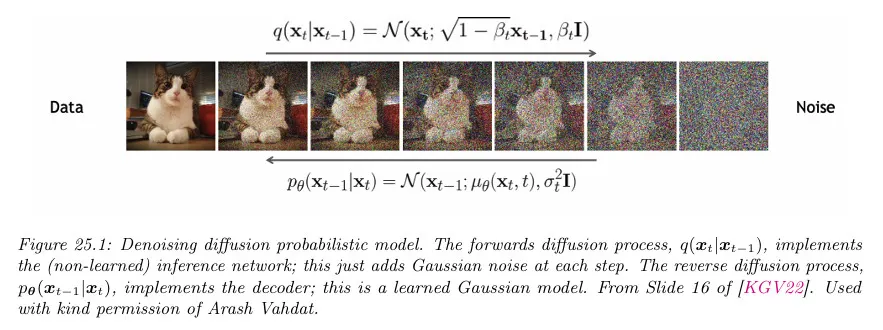
Denoising Diffusion Probabilistic Model (DDPM)
DDPM은 이미지를 생성하는데 노이즈 분포를 활용하는 모델이다. 이 모델은 이미지를 (가우시안) 노이즈 분포로 만드는 forward process를 수행한 후에, 해당 노이즈 분포에서 이미지를 복원(생성)하는 reverse process를 학습하여 이미지를 생성한다. 이때 각 단계에 추가되는 noise를 예측하고 그 예측된 noise 값을 현재 분포에서 제거하여 이미지를 복원(생성)한다. 이것은 각 단계에서 이미지를 복원하는 역함수를 사용하는 Normalizing Flow과 대비된다.
DDPM은 모든 잠재가 입력 와 동일한 차원을 갖는다는 점을 제외하면 Hierarchical Variational AutoEncoder(HVAE)와 유사한 것으로 생각할 수 있다. Normalizing Flow와도 유사하지만 Diffusion Model은 잠재 레이어가 확률적이고 역 변환을 사용할 필요가 없다.
Diffusion model에서 encoder 네트워크 는 학습되지 않는 단순 선형 가우시안 모델이고 decoder 네트워크 는 모든 시간 단계에 걸쳐 공유된다. 이러한 제한으로 학습 목적이 간단해져 posterior 붕괴의 위험 없이 심층 모델을 학습할 수 있다. Diffusion model의 학습은 일련의 weighted 비선형 최소 제곱 문제로 축소시킬 수 있다.
Diffusion model의 가장 핵심적인 부분은 결국 아래 정의되는 noise schedule만 이용해서 해당 시점의 샘플을 계산(forward pass)하거나 생성(reverse pass) 할 수 있다는 것이다. 이것은 모델이 가우시안 분포를 따른다는 가정과 Markov Chain을 따라 가우시안 노이즈가 추가된다는 설정 때문에 가능한데, 이 덕분에 timestep 별로 정답 샘플을 쉽게 생성할 수 있어서 높은 학습 효율을 가질 수 있게 되었고 현재 이미지 생성 분야에 주류 모델이 되었다.
Autoencoder 류의 모델은 원본 데이터를 저차원 Latent Space로 압축한 후에 그걸 다시 복원하는 과정을 통해 Latent Space가 원본 데이터를 복구하기 위한 feature —이것은 원본에 드러나지 않는 것일 수 있음— 를 학습하는 개념의 모델인 반면, DDPM은 원본 데이터를 순수 (가우시안) 노이즈로 변환했다가 그걸 다시 원본으로 단계별로 복구하는 과정을 통해 모델이 데이터에서 무엇이 noise이고 아닌지를 구분하는 능력을 학습하는 모델이라고 볼 수 있다. 참고로 Normalizing Flow는 원본 데이터를 단순한 (가우시안) 분포로 변환한 후에 그것을 역함수를 통해 다시 원래의 복잡한 분포로 단계별로 변환하는 과정을 통해 데이터 분포의 구조를 학습하는 모델이라고 할 수 있다.
Note) Diffusion Model이 라벨링 없이 원본 이미지만으로 chain을 따라 noise를 먹인 후에 denoising 단계에서 noise를 예측하여 각 단계별로 이미지의 representation을 학습한다는 개념은, SimCLR이나 BYOL, DINO 같은 self-supervised 모델에서 하나의 이미지를 서로 다르게 augmentation 시킨 후에, 다르게 augmentation 된 이미지를 예측(또는 대조) 하는 self-supervised learning과 근본적으로 동일하다. Diffusion Model은 chain을 통해 단계별로 예측하는 반면 기존의 self-supervised model은 다른 network에서 예측하거나 positive pair, negative pair로 대조하게 함. self-supervised learning은 라벨링 없이 원본만으로 학습이 가능하다는 점에서 저렴한 비용으로 대규모 데이터를 사용할 수 있고, 결과적으로 높은 성능을 발휘할 수 있다. 이렇게 보면 Diffusion Model은 학습 방법에 가까운 것이라 아키텍쳐는 자유롭게 선택할 수 있다. Diffusion Model은 decoder(forward pass는 계산되는 부분이니 생략)를 UNet을 사용하지만, ViT 같은 모델을 사용하는 것도 가능하다. 실제로 Video 생성 모델에서는 Diffusion 모델과 ViT를 섞어서 사용함.
Encoder (forwards diffusion)
Diffusion Model의 Encoder는 복잡한 이미지를 가우시안 분포로 변환하는 단계이다. 이것은 계산에 의해 가능하며, 학습되는 부분이 아니다.
형식적으로 Encoder는 다음의 단순 선형 가우시안 모델로 정의된다.
여기서 은 노이즈 스케쥴를 따라 선택된다.
입력에 조건화된 모든 잠재 상태에 대한 결합 분포는 다음과 같이 주어진다.
이것이 선형 가우시안 마르코프 체인을 정의하기 때문에 닫힌 형식으로 marginal을 계산할 수 있다.
우선 를 Reparametrization Trick을 사용하여 아래와 같이 표현할 수 있다.
여기서 다음을 정의하면
위의 reparametrization trick 식을 다음과 같이 전개할 수 있다.
따라서
위의 식에서 (*)은 분산이 다른 두 가우시안, 과 을 병합하면 새로운 분포는 이 된다는 것을 이용한다.
여기서 가 되도록 과 같은 노이즈 스케쥴을 고른다.
위의 식을 이용하면 입력을 체인을 따라 계산할 필요 없이 noise schedule만 이용해서 시점의 분포를 바로 계산할 수 있다.
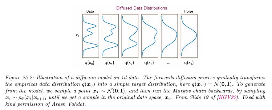
이 분포 를 diffusion kernel이라고 한다. 이것을 입력 데이터 분포에 적용한 다음 unconditional marginal을 계산하는 것은 가우시안 컨볼루션과 동등하다.
가 증가함에 따라 marginals은 더 단순해 진다. 아래 그림 참조. 이미지 도메인에서 이 절차는 우선 high-frequency(고주파) content(즉 텍스트와 같은 low-level detail)을 제거하고, 이후에 low-frequency(저주파) content(즉, shape 같은 high-level 또는 의미적 정보)를 제거한다.
Decoder (reverse diffusion)
Diffusion Model의 Decoder에서는 forward process를 반전해서 가우시안 노이즈에서 샘플을 생성하기를 원한다. 만일 입력 을 알면 의 한 단계 forward의 역 을 유도할 수 있다. 우선 조건부 확률에 대한 베이즈 룰을 사용하여
각 항을 대입하며 유도하면
여기서 는 를 포함하지 않는 함수이므로 생략한다. 표준 가우스 밀도 함수에 따라 평균과 분산을 다음과 같이 매개변수화할 수 있다.
가우시안 분포를 지수 안에 2차식 의 형태로 표현할 수 있으면 해당 2차식의 계수를 이용하여 평균과 분산을 구할 수 있음에 유의하라
아래와 같이 의 1차식의 계수를 2차식의 계수로 나눠서 평균을 구하고, 2차식의 계수의 역수를 이용해 분산을 구한다.
정리하면 아래와 같다.
그러나 새로운 데이터포인트를 생성할 때 를 모른다. 따라서 의 평균에 대해 위의 분포를 근사하도록 생성기를 훈련해야 한다. 이를 위해 다음 형식을 갖는 생성기를 선택한다.
종종 로 설정한다. 을 어떻게 학습하는지는 아래의 Model fitting에서 논의한다. 일단 자연스러운 2가지 선택은 reverse 프로세스 엔트로피에 대한 상한과 하한에 해당하는 와 이다.
모든 생성된 변수에 대한 해당 결합 분포는 다음과 같이 주어진다. 여기서 로 설정한다.
다음의 pseudocode를 사용하여 이 분포에서 샘플할 수 있다.
Algorithm: DDPM 모델에서 샘플링
1.
2.
foreach do
a.
b.
3.
반환
Model fitting
Diffusion Model은 VAE와 유사하게 Evidence Lower Bound(ELBO)를 최대화하여 모델을 맞춘다. 특히 각 데이터 예제 에 대해 다음의 log likelihood를 갖는다. (가 decoder이므로 는 생성된 이미지가 됨)
위 식에서 는 표기만 다를 뿐 와 동일한 의미이다. 종종 물리학에서 사용된다고 함. 이것은 에서 시작해서 시간 까지 확산된 모든 forward 경로에 대한 적분을 의미함.
는 reverse process에서 모델에 의해 생성된 전체 경로의 확률과 forward process의 전체 경로의 확률 사이의 비율을 의미한다.
결국 Decoder에 대한 likelihood는 forward pass의 전체 경로에 대한 적분을 reverse pass와 forward pass 사이의 비율과 곱한 것으로 정의된다. 거기에 최종적으로 log를 씌움.
이 log likelihood에 대한 ELBO는 다음과 같이 유도된다.
일반적으로 log가 적분 안으로 들어갈 수 없는데, 만일 함수가 convex이면 Jensen 부등식을 따라 log가 적분 안으로 들어가고 대신 부등호 기호로 바뀐다. 위 식의 2번째 줄은 이를 바탕으로 유도됨. 일반적으로 ELBO는 이러한 방법으로 유도한다.
그 다음 3번째 줄에서 전체 reverse process와 forward process의 비율을 각 timestep 별로 나누어 reverse, forward의 비율을 구한 후에 전체를 곱한 다음 reverse를 시작하기 위한 초기 조건인 를 곱하는 것으로 변경한다.
그리고 마지막 줄에서 적분을 기대값으로 변환한다.
이 ELBO에서 항을 계산하는 방법을 보기 위해 마르코프 속성으로 다음이 성립함을 확인한다.
또한 베이즈룰에 의해 다음이 성립한다.
이것을 위의 ELBO에 연결하여 다음을 얻는다.
으로 표시된 항은 telescoping 합으로 다음처럼 단순화될 수 있다.
따라서 negative ELBO(variational 상한)은 다음이 된다.
모든 분포가 가우시안이므로 이 KL 항의 각각이 해석적으로 계산될 수 있다. 처음과 마지막을 제외하고 아래에서는 항에 초점을 맞춘다. 이므로 를 이용하여 다음과 같이 작성할 수 있다.
따라서 노이즈 입력 가 주어지면 노이즈 제거된 의 평균을 예측하도록 모델을 학습하는 대신 다음과 같이 해당 시점의 노이즈를 예측하도록 모델을 학습하고 이로부터 평균을 계산할 수 있다. 아래 식 는 timestep 에서 이미지 의 평균을 의미하고, 그 내부의 는 모델이 해당 시점에 예측한 노이즈가 된다.
여기서 에 대한 의존성은 암시적이다. 다시 말해 모델을 시점의 노이즈를 예측하도록 학습 시킨 후에 그 구해진 노이즈 값을 적절히 조정해서 에서 빼면 을 구할 수 있다. 이렇게 하면 모델이 입력 과 에 대한 의존 없이 학습할 수 있다.
이 파라미터화를 사용하면 손실은 다음이 된다.
시간 종속 가중치 는 학습 목적이 maximum likelihood 학습에 해당하는 것을 보장한다. (variational bound가 타이트하다고 가정하여) 그러나 을 설정하면 모델이 더 보기 좋은 샘플을 생성한다는 것이 경험적으로 밝혀졌다. 결과적으로 단순화된 손실(또한 모델의 시간 단계 에 대한 평균화)은 다음과 같이 주어진다.
전체 학습 절차는 아래 pseudo code 참조. 더 진보된 가중치 스키마를 사용하면 샘플의 인지적 품질을 개선할 수 있다.
Algorithm: 을 사용하여 DDPM 모델 학습
1.
while 수렴할때까지 do
a.
b.
c.
d.
에 대해 gradient descent 단계를 취한다.
Noise Schedule
Diffusion Model의 Noise Schedule을 선형이나 cosine 같은 고정된 것을 사용하지 않고 최적화하는 접근을 Variational Diffusion Model(VDM)이라 한다. 이것은 다음의 인코더의 파라미터화를 사용한다.
와 를 독립적으로 작업하는 대신 그들의 비율을 예측하는 것을 학습한다. 이것을 signal to noise ratio(SNR, 신호대 잡음비)라고 한다.
이것은 에서 단조적으로 감소해야 하는데 다음을 정의하여 보장할 수 있다.
여기서 는 단조적 신경망이다. 일반적으로 분산 보존 SDE에 해당하는 를 설정한다.
Model fitting의 유도를 따라 negative ELBO를 다음처럼 작성할 수 있다.
여기서 처음 두 항은 표준 VAE와 유사하고 마지막 diffusion loss는 다음처럼 주어진다.
여기서 는 SNR 함수의 도함수이고 이다.
SNR 함수가 단조성 가정 때문에 가역이므로 change of variable을 수행할 수 있고 모든 것을 대신 의 함수로 만들 수 있다. 특히 이고 라 가정하면 위의 방정식을 다음처럼 재작성할 수 있다.
여기서 이다. 따라서 SNR 스케쥴의 모양은 2개의 끝점의 값을 제외하고 중요하지 않음을 알 수 있다.
위 방정식의 적분은 타임스텝을 랜덤으로 균일하게 샘플링하여 추정될 수 있다. 개 예제의 미니배치를 프로세싱할 때 low-discrepancy 샘플러를 사용하여 variational bound의 더 낮은 분산 추정을 생성할 수 있다. 이 접근에서 타임스텝을 독립적으로 샘플링하는 대신 단일 균등 랜덤 수 를 샘플링한 다음 번째 샘플에 대해 를 설정한다.
diffusion 손실의 분산에 관해 노이즈 스케쥴을 최적화할 수도 있다.
Sample Code
Model
Upsample, Downsample
우선 U-Net의 Encoder, Decoder에서 필요한 Upsample, Downsample 함수를 다음과 같이 정의한다. Upsample은 Upsample()을 통해 Upsampling을 하고 —그 뒤에 Conv2d()도 사용—, Downsample에서는 Conv2d()를 통해 downsampling을 한다.
def Upsample(dim, dim_out=None):
return nn.Sequential(
nn.Upsample(scale_factor=2, mode="nearest"),
nn.Conv2d(dim, default(dim_out, dim), 3, padding=1),
)
def Downsample(dim, dim_out=None):
# No More Strided Convolutions or Pooling
return nn.Sequential(
Rearrange("b c (h p1) (w p2) -> b (c p1 p2) h w", p1=2, p2=2),
nn.Conv2d(dim * 4, default(dim_out, dim), 1),
)
Python
복사
Position Embedding
위에서는 언급되지 않았지만 timestep 정보를 모델에 알려주기 위해 Sinusoidal Position Embedding을 수행한다. 이것은 Transformer의 Positional Encoding 방식을 참조한다.
# transformer의 positional encoding을 따라 time step을 embedding한다.
class SinusoidalPositionEmbeddings(nn.Module):
def __init__(self, dim):
super().__init__()
self.dim = dim
def forward(self, time):
device = time.device
half_dim = self.dim // 2
embeddings = math.log(10000) / (half_dim - 1)
embeddings = torch.exp(torch.arange(half_dim, device=device) * -embeddings)
embeddings = time[:, None] * embeddings[None, :]
embeddings = torch.cat((embeddings.sin(), embeddings.cos()), dim=-1)
return embeddings
Python
복사
WeightStandardizedConv2d
모델 내에서 일반적인 Conv2d 대신 Weighted Conv2d를 사용한다. 이것은 group normalization과 함께 더 잘 작동한다고 한다.
class WeightStandardizedConv2d(nn.Conv2d):
"""
https://arxiv.org/abs/1903.10520
weight standardization purportedly works synergistically with group normalization
"""
def forward(self, x):
eps = 1e-5 if x.dtype == torch.float32 else 1e-3
weight = self.weight
mean = reduce(weight, "o ... -> o 1 1 1", "mean")
var = reduce(weight, "o ... -> o 1 1 1", partial(torch.var, unbiased=False))
normalized_weight = (weight - mean) / (var + eps).rsqrt()
return F.conv2d(
x,
normalized_weight,
self.bias,
self.stride,
self.padding,
self.dilation,
self.groups,
)
Python
복사
ResnetBlock
U-Net의 각 layer는 2개의 ResNet과 1개의 Attention, 1개의 up/downsampling으로 수행된다. 그 중에서 ResNet은 아래처럼 WeightedStandardizedConv2d()와 GroupNorm(), SiLU()를 2번 수행하는 구성인데, 이 때문에 해당 함수를 모아 block을 구성하여 사용한다.
마지막에는 up/downsampling 여부에 따라 입력을 Conv2d()나 Identity()를 수행한 뒤, 2개 block을 통과한 결과와 합쳐서 반환한다.
추가로 time_embed를 받아서 scale_shift를 구하는 mlp(SiLU(), Linear())를 사용한다. 일반적으로 scale_shift는 입력에 대해 수행하지만, DDPM에서는 time_emb에 대해 scale_shift를 구하는데, 이를 통해 모델이 시간 단계에 따라 입력 데이터를 어떻게 처리할지를 학습하게 한다.
class ResnetBlock(nn.Module):
"""https://arxiv.org/abs/1512.03385"""
def __init__(self, dim, dim_out, *, time_emb_dim=None, groups=8):
super().__init__()
self.mlp = (
nn.Sequential(nn.SiLU(), nn.Linear(time_emb_dim, dim_out * 2))
if exists(time_emb_dim)
else None
)
self.block1 = Block(dim, dim_out, groups=groups)
self.block2 = Block(dim_out, dim_out, groups=groups)
self.res_conv = nn.Conv2d(dim, dim_out, 1) if dim != dim_out else nn.Identity()
def forward(self, x, time_emb=None):
scale_shift = None
# time_emb를 이용해서 scale_shift를 구한다. 이를 통해 모델이 시간에 따라 적절하게 반응하도록 학습됨.
if exists(self.mlp) and exists(time_emb):
time_emb = self.mlp(time_emb)
time_emb = rearrange(time_emb, "b c -> b c 1 1")
scale_shift = time_emb.chunk(2, dim=1)
h = self.block1(x, scale_shift=scale_shift)
h = self.block2(h)
return h + self.res_conv(x)
class Block(nn.Module):
def __init__(self, dim, dim_out, groups=8):
super().__init__()
self.proj = WeightStandardizedConv2d(dim, dim_out, 3, padding=1)
self.norm = nn.GroupNorm(groups, dim_out)
self.act = nn.SiLU()
def forward(self, x, scale_shift=None):
x = self.proj(x)
x = self.norm(x)
if exists(scale_shift):
scale, shift = scale_shift
x = x * (scale + 1) + shift
x = self.act(x)
return x
Python
복사
AttentionBlock, LinearAttentionBlock
이 방법에서 2가지 Attention 방식을 정의한다. 하나는 일반적인 Attention이고, 다른 하나는 Linear Attention으로 이것은 일반 attention이 시간과 메모리 요구사항이 시퀀스에 따라 2차적인 것에 반해 선형을 갖는다.
class Attention(nn.Module):
def __init__(self, dim, heads=4, dim_head=32):
super().__init__()
self.scale = dim_head**-0.5
self.heads = heads
hidden_dim = dim_head * heads
self.to_qkv = nn.Conv2d(dim, hidden_dim * 3, 1, bias=False)
self.to_out = nn.Conv2d(hidden_dim, dim, 1)
def forward(self, x):
b, c, h, w = x.shape
qkv = self.to_qkv(x).chunk(3, dim=1)
q, k, v = map(
lambda t: rearrange(t, "b (h c) x y -> b h c (x y)", h=self.heads), qkv
)
# 원래는 q, k를 곱한 결과를 dim_head의 제곱근으로 나누는데, 수치적 안정성을 위해 q를 우선 dim_head 제곱근으로 나눈 후에 k와 곱한다.
q = q * self.scale
sim = einsum("b h d i, b h d j -> b h i j", q, k)
# softmax()를 하기 전에 수치적 안정성 향상을 위해 현재 결과에서 최대값 amax()를 찾은 후 빼준다. 이렇게 하면 최대값은 0이 되고 나머지는 음수가 됨.
sim = sim - sim.amax(dim=-1, keepdim=True).detach()
attn = sim.softmax(dim=-1)
out = einsum("b h i j, b h d j -> b h i d", attn, v)
out = rearrange(out, "b h (x y) d -> b (h d) x y", x=h, y=w)
return self.to_out(out)
# 기존 attention의 변종.
# regular attention에서는 2차적인 시간과 메모리 요구 사항을 시퀀스 길이에 따라 선형으로 만든다.
class LinearAttention(nn.Module):
def __init__(self, dim, heads=4, dim_head=32):
super().__init__()
self.scale = dim_head**-0.5
self.heads = heads
hidden_dim = dim_head * heads
self.to_qkv = nn.Conv2d(dim, hidden_dim * 3, 1, bias=False)
self.to_out = nn.Sequential(nn.Conv2d(hidden_dim, dim, 1),
nn.GroupNorm(1, dim))
def forward(self, x):
b, c, h, w = x.shape
qkv = self.to_qkv(x).chunk(3, dim=1)
q, k, v = map(
lambda t: rearrange(t, "b (h c) x y -> b h c (x y)", h=self.heads), qkv
)
q = q.softmax(dim=-2)
k = k.softmax(dim=-1)
q = q * self.scale
context = torch.einsum("b h d n, b h e n -> b h d e", k, v)
out = torch.einsum("b h d e, b h d n -> b h e n", context, q)
out = rearrange(out, "b h c (x y) -> b (h c) x y", h=self.heads, x=h, y=w)
return self.to_out(out)
Python
복사
각 Attention을 GroupNorm()과 Residual과 함께 사용하기 위해 Block으로 만든다.
# Attention을 gruopNorm과 reset과 함께 사용하기 위해 block으로 만든다.
class AttentionBlock(nn.Module):
def __init__(self, dim):
super().__init__()
self.attn = Attention(dim)
self.norm = nn.GroupNorm(1, dim)
def forward(self, x):
return self.attn(self.norm(x)) + x
# Linear Attention을 gruopNorm과 reset과 함께 사용하기 위해 block으로 만든다.
class LinearAttentionBlock(nn.Module):
def __init__(self, dim):
super().__init__()
self.attn = LinearAttention(dim)
self.norm = nn.GroupNorm(1, dim)
def forward(self, x):
return self.attn(self.norm(x)) + x
Python
복사
U-Net
위의 building block을 합쳐서 U-Net을 구성한다.
class Unet(nn.Module):
def __init__(
self,
dim,
init_dim=None,
out_dim=None,
dim_mults=(1, 2, 4, 8),
channels=3,
self_condition=False,
resnet_block_groups=4,
):
super().__init__()
# determine dimensions
self.channels = channels
self.self_condition = self_condition
input_channels = channels * (2 if self_condition else 1)
init_dim = default(init_dim, dim)
self.init_conv = nn.Conv2d(input_channels, init_dim, 1, padding=0) # changed to 1 and 0 from 7,3
dims = [init_dim, *map(lambda m: dim * m, dim_mults)]
in_out = list(zip(dims[:-1], dims[1:]))
# time embeddings
time_dim = dim * 4
self.time_mlp = nn.Sequential(
SinusoidalPositionEmbeddings(dim),
nn.Linear(dim, time_dim),
nn.GELU(),
nn.Linear(time_dim, time_dim),
)
# layers
self.downs = nn.ModuleList([])
self.ups = nn.ModuleList([])
num_resolutions = len(in_out)
for ind, (dim_in, dim_out) in enumerate(in_out):
is_last = ind >= (num_resolutions - 1)
self.downs.append(
nn.ModuleList(
[
ResnetBlock(dim_in, dim_in, time_emb_dim=time_dim, groups=resnet_block_groups),
ResnetBlock(dim_in, dim_in, time_emb_dim=time_dim, groups=resnet_block_groups),
LinearAttentionBlock(dim_in),
Downsample(dim_in, dim_out) if not is_last else nn.Conv2d(dim_in, dim_out, 3, padding=1),
]
)
)
mid_dim = dims[-1]
self.mid_block1 = ResnetBlock(mid_dim, mid_dim, time_emb_dim=time_dim, groups=resnet_block_groups)
self.mid_attn = AttentionBlock(mid_dim)
self.mid_block2 = ResnetBlock(mid_dim, mid_dim, time_emb_dim=time_dim, groups=resnet_block_groups)
for ind, (dim_in, dim_out) in enumerate(reversed(in_out)):
is_last = ind == (len(in_out) - 1)
self.ups.append(
nn.ModuleList(
[
ResnetBlock(dim_out + dim_in, dim_out, time_emb_dim=time_dim, groups=resnet_block_groups),
ResnetBlock(dim_out + dim_in, dim_out, time_emb_dim=time_dim, groups=resnet_block_groups),
LinearAttentionBlock(dim_out),
Upsample(dim_out, dim_in) if not is_last else nn.Conv2d(dim_out, dim_in, 3, padding=1),
]
)
)
self.out_dim = default(out_dim, channels)
self.final_res_block = ResnetBlock(dim * 2, dim, time_emb_dim=time_dim, groups=resnet_block_groups)
self.final_conv = nn.Conv2d(dim, self.out_dim, 1)
def forward(self, x, time, x_self_cond=None):
if self.self_condition:
x_self_cond = default(x_self_cond, lambda: torch.zeros_like(x))
x = torch.cat((x_self_cond, x), dim=1)
x = self.init_conv(x)
r = x.clone()
t = self.time_mlp(time)
# skip connection을 위한 용도
h = []
for resnet1, resnet2, attn, downsample in self.downs:
x = resnet1(x, t)
h.append(x)
x = resnet2(x, t)
x = attn(x)
h.append(x)
x = downsample(x)
x = self.mid_block1(x, t)
x = self.mid_attn(x)
x = self.mid_block2(x, t)
for resenet1, resnet2, attn, upsample in self.ups:
x = torch.cat((x, h.pop()), dim=1)
x = resenet1(x, t)
x = torch.cat((x, h.pop()), dim=1)
x = resnet2(x, t)
x = attn(x)
x = upsample(x)
x = torch.cat((x, r), dim=1)
x = self.final_res_block(x, t)
return self.final_conv(x)
Python
복사
Sampling
Schedule
DDPM의 핵심인 Beta Schedule은 linear, quadratic, cosine 등 여러 형태가 가능하다.
def cosine_beta_schedule(timesteps, s=0.008):
"""
cosine schedule as proposed in https://arxiv.org/abs/2102.09672
"""
steps = timesteps + 1
x = torch.linspace(0, timesteps, steps)
alphas_cumprod = torch.cos(((x / timesteps) + s) / (1 + s) * torch.pi * 0.5) ** 2
alphas_cumprod = alphas_cumprod / alphas_cumprod[0]
betas = 1 - (alphas_cumprod[1:] / alphas_cumprod[:-1])
return torch.clip(betas, 0.0001, 0.9999)
def linear_beta_schedule(timesteps):
beta_start = 0.0001
beta_end = 0.02
return torch.linspace(beta_start, beta_end, timesteps)
def quadratic_beta_schedule(timesteps):
beta_start = 0.0001
beta_end = 0.02
return torch.linspace(beta_start**0.5, beta_end**0.5, timesteps) ** 2
def sigmoid_beta_schedule(timesteps):
beta_start = 0.0001
beta_end = 0.02
betas = torch.linspace(-6, 6, timesteps)
return torch.sigmoid(betas) * (beta_end - beta_start) + beta_start
Python
복사
정의된 Beta Schedule을 이용하여 alpha와 alpha_cumprod, posterior 분산을 아래처럼 구한다. 아래서는 timesteps = 300과 linear schedule을 사용했다.
timesteps = 300
# define beta schedule
betas = linear_beta_schedule(timesteps=timesteps)
# define alphas
alphas = 1. - betas
alphas_cumprod = torch.cumprod(alphas, axis=0)
alphas_cumprod_prev = F.pad(alphas_cumprod[:-1], (1, 0), value=1.0)
sqrt_recip_alphas = torch.sqrt(1.0 / alphas)
# calculations for diffusion q(x_t | x_{t-1}) and others
sqrt_alphas_cumprod = torch.sqrt(alphas_cumprod)
sqrt_one_minus_alphas_cumprod = torch.sqrt(1. - alphas_cumprod)
# calculations for posterior q(x_{t-1} | x_t, x_0)
posterior_variance = betas * (1. - alphas_cumprod_prev) / (1. - alphas_cumprod)
Python
복사
추가로 forward process와 reverse process에서 timestep에 해당하는 값을 추출하는 함수를 아래처럼 정의한다.
def extract(alphas, timesteps, x_shape):
batch_size = timesteps.shape[0]
out = alphas.gather(-1, timesteps.cpu()) # alphas에서 timestep의 index가 가리키는 값을 가져온다
return out.reshape(batch_size, *((1,) * (len(x_shape) - 1))).to(timesteps.device)
Python
복사
Forward process
원본을 noisy 이미지로 만드는 forward process에서 샘플을 생성하는 q_sample() 함수는 아래처럼 구현한다. 이 함수는 아래 식을 따른다.
# forward diffusion (using the nice property)
def q_sample(x_start, timesteps, noise=None):
if noise is None:
noise = torch.randn_like(x_start)
# sqrt_alphas_cumprod와 sqrt_one_minus_alphas_cumprod에서 현재 timestep에 해당하는 값을 가져온다.
sqrt_alphas_cumprod_t = extract(sqrt_alphas_cumprod, timesteps, x_start.shape)
sqrt_one_minus_alphas_cumprod_t = extract(sqrt_one_minus_alphas_cumprod, timesteps, x_start.shape)
# reparametrization trick을 이용하여 forward process에서 샘플 x_t를 계산
return sqrt_alphas_cumprod_t * x_start + sqrt_one_minus_alphas_cumprod_t * noise
Python
복사
Reverse proces
noisy 이미지에서 원본을 복구하는 reverse process에서 샘플을 생성하는 p_sample() 함수를 아래처럼 구현한다.
여기서 model의 평균은 아래 식을 따른다. 여기서 은 모델이 예측한 noise 값이므로 코드사에서 model의 forward 결과를 사용함.
최종 샘플은 reparametrization trick을 따라 위의 평균에 분산을 더해 구할 수 있다.
# reverse process에서 단일 샘플을 생성
@torch.no_grad()
def p_sample(model, x, timesteps, t_index):
# betas, sqrt_one_minus_alphas_cumprod, sqrt_recip_alphas에서 현재 timestep에 맞는 값을 가져온다.
betas_t = extract(betas, timesteps, x.shape)
sqrt_one_minus_alphas_cumprod_t = extract(sqrt_one_minus_alphas_cumprod, timesteps, x.shape)
sqrt_recip_alphas_t = extract(sqrt_recip_alphas, timesteps, x.shape)
# Equation 11 in the paper
# Use our model (noise predictor) to predict the mean
# reverse process에서 x_t에 대한 평균
# 모델의 예측 결과 model(x, timesteps)는 현재 timestep의 noise에 해당하고, 그 noise를 이용해서 해당 시점의 평균을 구한다.
model_mean = sqrt_recip_alphas_t * (x - betas_t * model(x, timesteps) / sqrt_one_minus_alphas_cumprod_t)
# timestep이 0이면 평균을 그대로 사용
if t_index == 0:
return model_mean
# timestep이 0이 아니면 reparametrization trick을 이용하여 현재 timestep의 분산을 더해서 샘플 x_t를 구한다.
else:
# posterior_variance에서 현재 timestep에 맞는 값을 가져온다.
posterior_variance_t = extract(posterior_variance, timesteps, x.shape)
noise = torch.randn_like(x)
# Algorithm 2 line 4:
return model_mean + torch.sqrt(posterior_variance_t) * noise
Python
복사
위의 p_sample()은 단일 샘플을 복구하는 것이고, 실제로는 여러 timestep을 반복하여 샘플을 복구하므로 아래와 같이 p_sample_loop()를 구현하여 샘플을 생성한다. 처음에는 noise에서 시작하고 반복문에서는 이전 sample을 다음 sample의 입력으로 사용한다.
# Algorithm 2 (including returning all images)
# reverse process에서 단일 샘플 생성을 연속으로 수행하여 최종 이미지를 생성한다.
@torch.no_grad()
def p_sample_loop(model, shape):
device = next(model.parameters()).device
b = shape[0]
# start from pure noise (for each example in the batch)
# 최초 샘플은 noise에서 시작
img = torch.randn(shape, device=device)
imgs = []
for i in tqdm(reversed(range(0, timesteps)), desc='sampling loop time step', total=timesteps):
# 이전 단계 샘플을 넣어서 새로운 샘플을 생성한다.
img = p_sample(model, img, torch.full((b,), i, device=device, dtype=torch.long), i)
imgs.append(img.cpu().numpy())
return imgs
Python
복사
Objective
샘플을 생성할 때는 평균과 분산을 이용하지만, 모델 자체는 noise를 예측하도록 훈련 받기 때문에 우선 noise를 랜덤으로 생성해서 forward process인 q_sample()을 수행한 후에 q_sample()에서 생성한 해당 noisy 입력을 모델에 넣어 모델이 예측한 noise를 얻고, 그 noise를 원래의 noise와 비교하여 손실을 구한다. 일반적으로 MSE를 사용하지만 l1 loss나 huber loss를 사용할 수도 있다.
# 모델이 최종적으로 noise를 예측하므로 원래 noise와 예측된 noise 사이의 손실을 구한다.
def p_losses(denoise_model, x_start, timesteps, noise=None, loss_type="l1"):
# forward 프로세스에 적용할 noise 생성
if noise is None:
noise = torch.randn_like(x_start)
# forward process를 통해 noisy 이미지를 구한다
x_noisy = q_sample(x_start=x_start, timesteps=timesteps, noise=noise)
# noisy 이미지와 timestep을 이용해서 모델이 noise를 예측한다
predicted_noise = denoise_model(x_noisy, timesteps)
# 실제 noise와 모델이 예측한 predicted_noise 사이의 loss 계산
if loss_type == 'l1':
loss = F.l1_loss(noise, predicted_noise)
elif loss_type == 'l2':
loss = F.mse_loss(noise, predicted_noise)
elif loss_type == "huber":
loss = F.smooth_l1_loss(noise, predicted_noise)
else:
raise NotImplementedError()
return loss
Python
복사
Train
위의 모델과 함수들을 이용하여 모델 생성하고 학습하는 코드는 아래 참조. optimizer는 Adam을 사용하고 학습 과정을 기록하기 위해 중간에 이미지를 저장한다. 학습 된 모델을 이용해서 실제 이미지를 얻으려면 p_sample_loop()을 사용하면 된다.
from torch.optim import Adam
from torchvision.utils import save_image
device = "cuda" if torch.cuda.is_available() else "cpu"
print("device: ", device)
model = Unet(
dim=image_size,
channels=channels,
dim_mults=(1, 2, 4,)
)
model.to(device)
optimizer = Adam(model.parameters(), lr=1e-3)
results_folder = Path("./results")
results_folder.mkdir(exist_ok = True)
save_and_sample_every = 1000
epochs = 6
for epoch in range(epochs):
for step, batch in enumerate(dataloader):
optimizer.zero_grad()
batch_size = batch["pixel_values"].shape[0]
batch = batch["pixel_values"].to(device)
# Algorithm 1 line 3: sample t uniformally for every example in the batch
t = torch.randint(0, timesteps, (batch_size,), device=device).long()
loss = p_losses(model, batch, t, loss_type="huber")
if step % 100 == 0:
print("Loss:", loss.item())
loss.backward()
optimizer.step()
# save generated images
if step != 0 and step % save_and_sample_every == 0:
milestone = step // save_and_sample_every
batches = num_to_groups(4, batch_size)
all_images_list = list(map(lambda n: p_sample_loop(model, shape=(n, channels, image_size, image_size)), batches))
all_images = torch.cat(all_images_list, dim=0)
all_images = (all_images + 1) * 0.5
save_image(all_images, str(results_folder / f'sample-{milestone}.png'), nrow = 6)
Python
복사
